Appearance
4.1 — What a Signal Is, and the Kinds There Are
A signal is a function that carries information. The voltage from a microphone as a function of time. The brightness of a photograph as a function of position. The daily closing price of a share. All three are signals, and the same mathematics handles all three, which is the reason this Part exists as a subject rather than as an appendix to circuit theory.
The classification below looks like taxonomy for its own sake. It is not: each distinction decides which tools apply. Whether a signal is periodic decides between Fourier series and Fourier transform. Whether it has finite energy decides whether its transform exists at all. Whether it is continuous or discrete decides between Laplace and Z.
The mathematics behind this Part is Volume II Part 9, and the physical waves it describes are Volume IV Part 2. This chapter is the vocabulary that sits between them: what counts as a signal, and which of its properties decide what you are allowed to do to it.
1. Continuous time and discrete time
A continuous-time signal is defined for every instant. Written x(t), with round brackets and t a real number.
A discrete-time signal is defined only at integer indices. Written x[n], with square brackets and n an integer. The bracket convention is universal and carries real meaning — square brackets mean the signal simply does not exist between samples, not that it is zero there.
x[n] usually comes from sampling x(t) at intervals T_s:
x[n] = x(nT_s)
Do not confuse discrete-time with digital. Discrete time means the time axis is a set of points. Digital means the amplitude is quantised to a finite set of values as well. A sampled but unquantised signal — the output of a sample-and-hold circuit from Chapter 3.5 — is discrete in time and continuous in amplitude. Digital requires both.
| Continuous amplitude | Discrete amplitude | |
|---|---|---|
| Continuous time | analog | rare, e.g. a quantised sensor output |
| Discrete time | sampled | digital |
The difference between the two is easiest to see when one is made from the other.
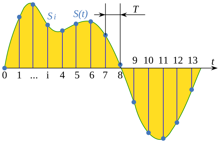
Read the two carefully, because the difference is not a matter of appearance only. The smooth curve has a value at every one of infinitely many instants. The stems have values at a countable set of instants and are undefined between them — not zero, undefined. Asking a discrete signal what it was doing halfway between two samples is a question with no answer, which is why the reconstruction problem in Chapter 4.7 is a real problem rather than a formality.
The spacing between stems is the sampling interval T_s, and its reciprocal f_s = 1/T_s is the sampling rate. Those two symbols run through the rest of this Part and all of Part 5, and they mean exactly what the picture shows: how far apart the stems are, and how many of them per second.
2. Periodic and aperiodic
A signal is periodic if it repeats exactly:
x(t) = x(t+T) \quad\text{for all } t
The smallest positive T that works is the fundamental period, and f_0 = 1/T is the fundamental frequency.
For discrete time the condition is x[n] = x[n+N] with N an integer, and that integer requirement causes a genuine surprise. Consider x[n] = \cos(\omega_0 n). For periodicity you need
\cos(\omega_0 n) = \cos(\omega_0 n + \omega_0 N)
which requires \omega_0N = 2\pi k for some integer k, so
\frac{\omega_0}{2\pi} = \frac{k}{N} \quad\text{must be rational}
A discrete-time sinusoid is periodic only if its frequency is a rational fraction of 2\pi. So \cos(n/6) — a perfectly reasonable-looking signal — is not periodic at all, because 1/(12\pi) is irrational. Its continuous cousin \cos(t/6) is periodic with period 12\pi. Sampling destroyed the periodicity.
This is not a curiosity. It is why a digital oscillator's output repeats only if you choose the frequency ratio carefully, and it is why a musical note synthesised digitally at an awkward frequency has a phase that drifts through the waveform table.
Adding periodic signals
Add two periodic signals with periods T_1 and T_2 and the sum is periodic only if T_1/T_2 is rational; the combined period is then the least common multiple.
Worked example. \cos(2\pi\cdot 3t) + \cos(2\pi\cdot 5t) has periods 1/3 and 1/5. Their ratio is 5/3, rational, so the sum is periodic with period 1 — the least common multiple of 1/3 and 1/5. The fundamental frequency of the sum is 1 Hz, even though neither component is at 1 Hz. That "missing fundamental" is a real perceptual phenomenon: play the harmonics of a low note without the note itself and the ear still hears the pitch of the fundamental, which is why a small radio speaker that cannot reproduce 60 Hz still conveys bass.
3. Energy and power signals
The energy of a signal is defined by analogy with a resistor dissipating v^2/R, taking R=1:
E = \int_{-\infty}^{\infty}|x(t)|^2\,dt \qquad\text{or}\qquad E = \sum_{n=-\infty}^{\infty}|x[n]|^2
Read aloud: "the integral from minus infinity to infinity of the magnitude of x of t squared, dee t."
The average power is the energy per unit time:
P = \lim_{T\to\infty}\frac{1}{2T}\int_{-T}^{T}|x(t)|^2\,dt
These give a clean and useful classification:
- An energy signal has finite energy and therefore zero average power. Anything that dies away: a single pulse, a decaying exponential, the sound of one handclap.
- A power signal has infinite energy and finite non-zero power. Anything that goes on forever: a sine wave, a square wave, a constant, noise.
No signal can be both, and some signals are neither (x(t) = t has infinite power as well as infinite energy).
Why it matters: the Fourier transform of Chapter 4.4 converges for energy signals but not for power signals. Sines and constants need the transform to be extended with impulse functions, and periodic signals get their own tool, the Fourier series. The classification tells you which chapter to open.
Worked example. For x(t) = e^{-at}u(t) with a>0, where u(t) is the step function of section 5:
E = \int_0^\infty e^{-2at}dt = \left[\frac{e^{-2at}}{-2a}\right]_0^\infty = \frac{1}{2a}
Finite, so it is an energy signal.
For a sine x(t)=A\cos(\omega t):
P = \frac{1}{T}\int_0^T A^2\cos^2(\omega t)dt = \frac{A^2}{2}
using the same \overline{\cos^2}=\tfrac12 result as Chapter 1.6. Finite power, infinite energy — a power signal. And A^2/2 is exactly V_{rms}^2, which is why rms values and signal power are the same idea seen twice.
4. Even, odd, and the decomposition
\text{Even: } x(-t)=x(t) \qquad \text{Odd: } x(-t)=-x(t)
Even signals are symmetric about the vertical axis, like a cosine. Odd signals are antisymmetric, like a sine.
Any signal splits uniquely into an even part and an odd part:
x_e(t) = \frac{x(t)+x(-t)}{2}, \qquad x_o(t)=\frac{x(t)-x(-t)}{2}
Check that these add back: x_e+x_o = \frac{x(t)+x(-t)+x(t)-x(-t)}{2} = x(t) ✓. And check the symmetries: replacing t by -t in x_e swaps the two terms in the numerator, giving the same thing ✓; doing the same in x_o negates it ✓.
Why this is useful: the Fourier transform of an even real signal is purely real, and of an odd real signal is purely imaginary. So the decomposition tells you the structure of the spectrum before you compute anything, and it halves the work in many derivations.
5. The standard test signals
Six functions do almost all the work in this Part. Each exists because it isolates one aspect of a system's behaviour.
The unit step
u(t) = \begin{cases}1 & t\ge0\\0 & t\lt0\end{cases}
Models switching something on. Its value exactly at t=0 is a matter of convention and never affects an integral.
Its use: the step response of a system tells you about overshoot, settling time and steady-state error, which is why Chapter 6.3 is built entirely around it.
Any finite-duration pulse is built from steps: a pulse from t=2 to t=5 is u(t-2)-u(t-5).
The unit impulse
\delta(t) = 0 \text{ for } t\ne0, \qquad \int_{-\infty}^{\infty}\delta(t)\,dt = 1
Infinitely tall, infinitely narrow, unit area. This is not a function in the ordinary sense — no genuine function is zero everywhere except one point and yet integrates to 1. It is a distribution, and it is defined by what it does inside an integral rather than by its values.
Paul Dirac introduced it in the 1920s for quantum mechanics and was criticised by mathematicians for years. Laurent Schwartz built the rigorous theory of distributions in the 1940s, which won him the Fields Medal and made Dirac's usage legitimate. Engineers had been using it successfully throughout.
The sifting property is the only thing you actually need:
\int_{-\infty}^{\infty}x(t)\delta(t-t_0)\,dt = x(t_0)
In words: multiplying by a shifted impulse and integrating picks out the signal's value at that instant. The impulse "sifts" one value out of the whole function. Chapter 4.3 builds convolution directly on this.
The step and the impulse are related by calculus:
\delta(t)=\frac{du(t)}{dt}, \qquad u(t)=\int_{-\infty}^{t}\delta(\tau)\,d\tau
The derivative of a step is an impulse — the step's slope is zero everywhere except at the jump, where it is infinite, with the area under that infinity being exactly the jump's height.
In discrete time it is far less exotic:
\delta[n]=\begin{cases}1 & n=0\\0&\text{otherwise}\end{cases}
Just a 1 at index zero. No infinities, no distribution theory. This is one of several reasons discrete-time signal processing is mathematically easier than continuous-time, and worth remembering when Chapter 4.6 seems simpler than Chapter 4.5.
The ramp
r(t)=t\,u(t)
The integral of the step. Used to test whether a control system can track a steadily increasing input without falling behind — Chapter 6.3 shows which systems can and which cannot.
The exponential
x(t)=Ae^{st}, \qquad s=\sigma+j\omega
The single most important signal in this volume, and it is worth seeing why. Expanding with Euler's formula:
Ae^{(\sigma+j\omega)t}=Ae^{\sigma t}\left[\cos\omega t+j\sin\omega t\right]
One expression contains everything: with \sigma=0 it is a pure sine; with \omega=0 it is a pure exponential rise or decay; with both, it is a decaying or growing oscillation, exactly the RLC ringing of Chapter 1.5.
Its importance is this: the complex exponential is the one signal that passes through a linear time-invariant system unchanged in shape. Put e^{st} in and you get H(s)e^{st} out — the same exponential, scaled by a complex number. Nothing else does that. Chapter 4.3 proves it, and every transform in this Part is built on it.
The sinusoid
x(t)=A\cos(\omega t+\phi)
The special case \sigma=0, and the one you can actually generate and measure. Everything about phasors in Chapter 1.6 was this signal handled with the exponential's machinery.
The sinc
\text{sinc}(t)=\frac{\sin(\pi t)}{\pi t}
Equal to 1 at t=0 (by the limit, since \sin x \approx x for small x), zero at every non-zero integer, with decaying ripples either side.
It appears in two guises and they are the same fact: it is the Fourier transform of a rectangular pulse, and it is the ideal reconstruction filter's impulse response in Chapter 4.7. A perfect brick-wall filter in frequency is a sinc in time, and the sinc's infinite extent is exactly why a perfect filter cannot be built.
6. Operations on signals
Four transformations, and the order in which you apply them is a genuine trap.
Time shift. x(t-t_0) shifts right (later) by t_0 when t_0 is positive. This feels backwards and is not: at t=t_0 the argument is 0, so the value that used to happen at 0 now happens at t_0. Delay is a minus sign in the argument.
Time reversal. x(-t) flips the signal about the vertical axis.
Time scaling. x(at) compresses by a factor a when a>1, and stretches when a<1. Again inverted from intuition, for the same reason.
Amplitude operations — adding, multiplying, scaling — are pointwise and hold no traps.
The order trap
Sketch x(2t+4). There are two ways and only one is right.
Wrong: shift left by 4, then compress by 2. This gives x(2t) shifted by 4, which is x(2(t+4)) = x(2t+8).
Right: either
- factor first as x(2(t+2)), then compress by 2 and shift left by 2, or
- shift first by 4 to get x(t+4), then compress the whole thing by 2.
The reliable rule: always factor the argument into the form x(a(t-t_0)) first, and then the shift is unambiguously t_0 and the scale is unambiguously a. Check with one point: the original x(t) at t=0 should appear where 2t+4=0, that is t=-2 ✓ — matching the factored form's shift of -2.
7. Signals as vectors, briefly
A idea that pays off repeatedly later. Treat a signal as a vector in an infinite-dimensional space, with the inner product
\langle x,y\rangle = \int_{-\infty}^{\infty}x(t)y^*(t)\,dt
where the asterisk means complex conjugate. Then:
- Energy is the squared length of the vector, E = \langle x,x\rangle.
- Two signals are orthogonal when their inner product is zero — they share nothing.
- The Fourier series is a projection onto an orthogonal basis of sines and cosines, exactly like resolving a vector into x and y components.
Why \sin and \cos at harmonically related frequencies form an orthogonal set:
\int_0^T\cos(m\omega_0t)\cos(n\omega_0t)\,dt = 0 \quad\text{whenever } m\ne n
Prove it in one line with the product-to-sum identity: \cos A\cos B = \tfrac12[\cos(A-B)+\cos(A+B)], and both resulting cosines complete a whole number of cycles over T, so both integrate to zero.
That single orthogonality result is the entire mathematical basis of Fourier analysis, and it is why Chapter 4.4's coefficient formula works: to find how much of frequency n a signal contains, take its inner product with frequency n, and every other frequency contributes exactly zero.
Volume II, Chapter 4.1 develops the vector-space view properly; here it is enough to know that the analogy is exact, not decorative.
Signals are now classified and named. The next chapter asks what a system is, and identifies the two properties — linearity and time-invariance — that make everything else in this Part possible.
Every formula above, built from scratch
None of the results in this chapter are worth memorising, because each one can be rebuilt in under a minute from something simpler. What follows is that rebuilding, one result at a time, so the formula and the reason for it sit on the same page as the explanation that needed them.
Signal measures
E=\int_{-\infty}^{\infty}|x(t)|^2dt = \sum_n|x[n]|^2
P=\lim_{T\to\infty}\frac{1}{2T}\int_{-T}^{T}|x(t)|^2dt
An energy signal has finite E and zero P; a power signal has infinite E and finite P. No signal is both.
For a sinusoid of amplitude A: P = A^2/2, which is V_{rms}^2 — the same quantity as Chapter 1.6's rms, arrived at from the signals side.
x_e(t)=\frac{x(t)+x(-t)}{2}, \qquad x_o(t)=\frac{x(t)-x(-t)}{2}
Check: adding them gives x(t); substituting -t leaves x_e unchanged and negates x_o.
Periodicity in discrete time
x[n]=\cos(\omega_0n) \text{ is periodic} \iff \frac{\omega_0}{2\pi}=\frac kN \text{ is rational}
Derivation: periodicity needs \omega_0N=2\pi k for integers N and k, which rearranges to the stated condition. Continuous sinusoids have no such restriction.
Standard signals
u(t)=\begin{cases}1&t\ge0\\0&t\lt0\end{cases}, \qquad \delta(t)=\frac{du}{dt}, \qquad u(t)=\int_{-\infty}^t\delta(\tau)d\tau
\int_{-\infty}^{\infty}x(t)\delta(t-t_0)dt=x(t_0) \qquad\text{(sifting)}
\text{sinc}(t)=\frac{\sin\pi t}{\pi t}, \qquad \text{sinc}(0)=1, \qquad \text{sinc}(n)=0 \text{ for integer } n\ne0
Why sinc(0) = 1: for small x, \sin x\approx x, so \sin(\pi t)/(\pi t)\to1.