Appearance
5.5 — Image Processing
An image is a signal whose independent variable is position rather than time. Everything from Part 4 carries across — convolution, the Fourier transform, sampling, aliasing — with one axis becoming two.
Two things genuinely change. Nothing is causal, because there is no reason a filter cannot look to the right as well as the left. And the human visual system has its own peculiarities, which drive image compression just as hearing drove audio compression in Chapter 5.4.
1. How an image is represented
A grayscale image is a function f(x,y) giving intensity at each position, sampled onto a grid of pixels. Eight bits per pixel gives 256 levels, which is enough that ordinary photographs show no banding — although smooth gradients in a clear sky do, which is why 10-bit displays exist.
Colour needs three numbers per pixel. The obvious choice is red, green and blue, which matches how displays emit and how sensors detect. But RGB is a poor choice for processing and compression, for a reason that comes from the eye.
YCbCr separates brightness from colour:
Y = 0.299R+0.587G+0.114B
C_b = 0.564(B-Y), \qquad C_r=0.713(R-Y)
Y is luma, the brightness. C_b and C_r are chroma, the colour differences.
Look at the weights in the Y formula. Green counts for 59%, red for 30%, blue for only 11%. That is not arbitrary — it reflects the eye's sensitivity, which peaks in the green and is poor in the blue.
And the consequence that every image and video format exploits: the eye has far better spatial resolution for brightness than for colour. So the chroma channels can be sampled at half or quarter resolution with almost no visible loss.
- 4:4:4 — no reduction.
- 4:2:2 — chroma halved horizontally. Broadcast and professional video.
- 4:2:0 — chroma halved in both directions, so a quarter of the samples. JPEG, MPEG, and essentially all consumer video.
4:2:0 discards half the total data before any compression algorithm has run, and it is nearly invisible. The exception is fine coloured detail — red text on a blue background is where you see the artifacts, which is why screen recordings of code look worse than video of a face.
2. Point operations
Operations on each pixel independently, ignoring its neighbours.
Brightness and contrast:
g(x,y)=\alpha f(x,y)+\beta
\alpha scales contrast; \beta shifts brightness. Both can push values outside the valid range, so they must be clipped, and clipped values are lost permanently.
Gamma correction:
g = 255\left(\frac{f}{255}\right)^{1/\gamma}
This one deserves explaining, because it is universally present and rarely understood. Cathode ray tubes had a non-linear response — output brightness went roughly as input voltage to the power 2.2 — so cameras applied the inverse to compensate. CRTs are gone; the convention stayed, and for a good reason.
Human brightness perception is also roughly a power law, with an exponent near 0.45 — which is close to 1/2.2. So the gamma-encoded signal happens to be perceptually uniform: equal steps in the stored number are equal steps in apparent brightness. That makes 8 bits enough. Store light linearly in 8 bits and the dark tones would band badly, because the eye can distinguish far more shades in the dark than a linear scale allocates there.
The trap: most image processing mathematics assumes linear light. Blending, resizing and blurring gamma-encoded values gives subtly wrong results — a blurred edge between black and white comes out too dark. Correct procedure is to convert to linear, process, and convert back, which a great deal of software still does not do.
Histogram equalisation redistributes intensities so that all levels are used roughly equally, using the cumulative distribution of the existing histogram as the mapping. It reveals detail in a low-contrast image, and it exaggerates noise in flat areas, which is why the local variant CLAHE — applied to small tiles with a contrast limit — is what medical imaging actually uses.
3. Spatial filtering — two-dimensional convolution
g(x,y)=\sum_{i}\sum_{j}h(i,j)f(x-i,y-j)
The same operation as Chapter 4.3 with a second index. The filter h is called a kernel, and it is usually a small square: 3×3, 5×5, 7×7.
Smoothing
Box blur — all coefficients equal, summing to 1:
\frac19\begin{bmatrix}1&1&1\\1&1&1\\1&1&1\end{bmatrix}
Cheap and poor. Its frequency response is a two-dimensional sinc with substantial sidelobes, which produce visible ringing and a characteristic boxy look.
Gaussian blur:
h(i,j)=\frac{1}{2\pi\sigma^2}e^{-(i^2+j^2)/2\sigma^2}
The right smoothing filter, for three reasons. Its transform is another Gaussian, so there are no sidelobes and no ringing. It is separable — a 2D Gaussian equals a horizontal 1D Gaussian followed by a vertical one — so an n\times n kernel costs 2n operations per pixel instead of n^2. For a 15×15 kernel that is 30 operations instead of 225, a factor of seven. And it is the only filter that introduces no new detail at any scale, which is the formal property that makes it the correct choice for scale-space analysis.
Median filter. Replace each pixel with the median of its neighbourhood. Not a convolution at all — it is non-linear, so none of Part 4's theory applies.
But it does something no linear filter can. It removes salt-and-pepper noise — isolated black and white pixels — perfectly, because an outlier is never the median. And it preserves edges exactly, because at an edge the median is still one of the two genuine values, whereas a blur produces the average of them.
The general lesson worth carrying: when a linear filter cannot do what you need, the answer is often a rank-order or otherwise non-linear operation, and you give up the transform-domain machinery in exchange.
Edge detection
An edge is a rapid intensity change, so edge detection is differentiation.
Sobel kernels approximate the horizontal and vertical derivatives:
G_x=\begin{bmatrix}-1&0&1\\-2&0&2\\-1&0&1\end{bmatrix}, \qquad G_y=\begin{bmatrix}-1&-2&-1\\0&0&0\\1&2&1\end{bmatrix}
Read the structure. G_x subtracts the left column from the right — a horizontal difference. The middle row is weighted 2 because it is nearest the pixel of interest, which builds in a small vertical smoothing that makes the operator far less noise-sensitive than a plain difference.
|G|=\sqrt{G_x^2+G_y^2}, \qquad \theta=\arctan\frac{G_y}{G_x}
Laplacian — the second derivative, isotropic (no preferred direction):
\nabla^2=\begin{bmatrix}0&1&0\\1&-4&1\\0&1&0\end{bmatrix}
Edges appear as zero crossings, where the second derivative changes sign. More precise localisation than the first derivative, and much more sensitive to noise — so it is always preceded by a Gaussian blur, giving the Laplacian of Gaussian.
Canny edge detection — the standard, from John Canny's 1986 work, and worth knowing as a five-step pipeline because each step fixes a specific failure:
- Gaussian blur — because differentiating noise gives noise.
- Sobel gradients — magnitude and direction.
- Non-maximum suppression — thin the thick gradient ridges down to one-pixel lines by keeping only local maxima along the gradient direction.
- Double thresholding — mark strong edges and weak edges separately.
- Hysteresis — keep a weak edge only if it connects to a strong one.
Step 5 is the clever one and it is the same idea as the Schmitt trigger of Chapter 2.5. A single threshold either breaks real edges where they dip below it or admits noise where it rises above. Two thresholds plus connectivity keeps continuous edges intact while rejecting isolated noise.
Sharpening
g = f + \lambda(f - \text{blur}(f))
Read it: take the image, subtract a blurred version to get just the detail, and add that detail back amplified.
This is unsharp masking, and the name is a genuine relic of darkroom practice — a blurred (unsharp) negative was sandwiched with the original to produce the effect chemically, decades before computers.
It cannot recover lost detail. It amplifies what is there, and it amplifies noise along with it, and pushed too far it produces halos around edges. Every sharpening slider in every photo application is this operation, and the halos are how you spot an over-processed image.
The operation below is the same convolution as Chapter 4.3, with one difference: the sliding window now slides in two directions instead of one.
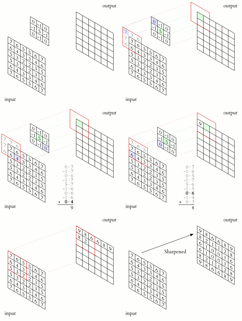
Follow one step of the animation. The kernel sits over a patch of the image. Each kernel number multiplies the pixel underneath it, all the products are added, and that single total becomes one pixel of the output. Then the kernel moves one pixel across and the whole thing repeats.
That is the entire operation, and every filter in this section is the same loop with different numbers in the kernel. A kernel of nine values all equal to 1/9 averages each pixel with its neighbours, which blurs. A kernel with a positive centre and negative surround measures how much a pixel differs from its neighbours, which sharpens and finds edges. Nothing about the code changes — only the numbers do, which is why image filtering is one function and a library of kernels.
The cost is worth noting too. A k\times k kernel over an N\times N image is k^2N^2 multiplications, so a 5×5 kernel over a 12-megapixel photo is 300 million of them. That is why this operation is the thing GPUs were built to do, and why the same loop reappears as the convolutional layer of a neural network in Volume I, Chapter 12.
4. The frequency domain in two dimensions
F(u,v)=\sum_x\sum_yf(x,y)e^{-j2\pi(ux/M+vy/N)}
Separable, so it is computed as an FFT of every row followed by an FFT of every column. Cost is O(MN\log MN).
Reading a 2D spectrum:
- The centre is DC — the average brightness.
- Distance from the centre is spatial frequency: near the centre is smooth gradients, far out is fine detail.
- Direction from the centre is the orientation of the pattern. A pattern of vertical stripes produces energy along the horizontal axis, because the intensity varies horizontally.
What this makes easy: removing a periodic pattern — scanner banding, halftone screen dots from a printed original, interference in a microscope image — is a matter of finding the bright spots away from the centre and zeroing them. No spatial filter can do that cleanly, and in the frequency domain it is a few clicks.
5. JPEG, step by step
Chapter 5.4 followed an MP3 encoder; JPEG is the same story with the eye in place of the ear, and the parallels are exact.
Step 1 — convert to YCbCr and subsample chroma to 4:2:0. Half the data is gone before anything else has happened.
Step 2 — split into 8×8 blocks. Each is processed independently, which is where the artifacts come from.
Step 3 — 2D DCT of each block. Sixty-four pixel values become sixty-four frequency coefficients. The top-left coefficient is the block's average brightness (DC); moving right and down means finer detail.
The DCT rather than the DFT for the reason Chapter 5.1 gave: it mirrors rather than wraps at the block boundary, so it avoids the artificial discontinuity and concentrates energy into fewer coefficients.
Step 4 — quantise. This is where the loss happens, and only here. Divide each coefficient by an entry from an 8×8 quantisation table and round.
The table has small values at the top left and large ones at the bottom right, so high frequencies are quantised coarsely and often to zero. The standard tables were derived from experiments on what people can see, exactly as MP3's masking curves were derived from what people can hear.
The quality setting scales the whole table. Quality 90 divides the table by a small factor, quality 30 multiplies it, and at quality 10 nearly everything below the first few coefficients becomes zero.
Step 5 — zig-zag scan. Read the 8×8 block in a diagonal zig-zag from the top left. This orders the coefficients roughly from low to high frequency, so all the zeros end up together in a long run at the end — which is exactly what the next step needs.
Step 6 — run-length and Huffman encode. Long runs of zeros compress to almost nothing, and the remaining values get variable-length codes.
The artifacts
- Blocking. Each 8×8 block is quantised independently, so adjacent blocks end up with slightly different average brightness and the grid becomes visible. This is the fundamental flaw of block-based coding, and JPEG 2000's wavelet transform (Chapter 5.3) eliminates it by not using blocks at all.
- Ringing. Sharp edges need high frequencies; quantising them coarsely produces the Gibbs overshoot of Chapter 4.4 as a halo. Text and line art suffer badly, which is why screenshots should be PNG and photographs should be JPEG.
- Colour bleeding. From the 4:2:0 subsampling, most visible on saturated red against blue.
Typical results
| Quality | Ratio | Verdict |
|---|---|---|
| 100 | 3:1 | indistinguishable |
| 90 | 10:1 | indistinguishable in normal viewing |
| 75 | 20:1 | good, the sensible default |
| 50 | 30:1 | visible on close inspection |
| 10 | 100:1 | badly broken |
Generation loss is real. Each save-and-reopen requantises coefficients that were already quantised, and because the DCT is not applied to exactly the same pixel values, errors accumulate. Editing a JPEG repeatedly destroys it. Work in a lossless format and export to JPEG once, at the end.
6. Video compression, briefly
Video adds one enormous redundancy that still images do not have: consecutive frames are nearly identical.
Motion compensation exploits it. Divide the frame into blocks; for each, search the previous frame for the best match; store only the motion vector saying where it came from and the small residual difference. A camera panning across a static scene produces almost no data at all, because every block is found unchanged a few pixels away.
The frame types:
- I-frame — encoded independently, like a JPEG. Needed so playback can start or seek.
- P-frame — predicted from the previous frame. Typically a tenth the size.
- B-frame — predicted from both previous and following frames, so it must be decoded out of order. Smallest of all.
B-frames are why a video file's frames are stored in a different order than they are displayed, and why seeking in a compressed video jumps to the nearest I-frame rather than the exact frame you asked for.
Rate control decides how many bits each frame gets. Constant bit rate keeps the data rate fixed and lets quality vary — necessary for broadcast. Constant quality lets the rate vary and gives a better result for the same average size — which is what streaming uses, since the network can buffer.
7. Where image processing meets learning
Everything above is hand-designed. Since about 2012 the dominant approach has been to learn the filters instead.
A convolutional neural network is, in its first layers, exactly the convolution of section 3 — except the kernel values are learned from data rather than chosen by a person. And what the first layer learns, reliably, across every network and every dataset, is edge detectors at various orientations, which look strikingly like Sobel kernels.
That is worth sitting with. Decades of hand-designed image processing converged on Gaussian smoothing followed by oriented derivatives, and a network given only data and a training objective arrives at the same operators independently. It is a strong argument that those operators are not conventions but the right answer to the problem.
Where learned methods now win outright: denoising, super-resolution, deblurring, and segmentation. Where classical methods still win: anything needing a guarantee, anything with no training data, anything that must run on a microcontroller, and anything where you must be able to explain what the algorithm did and why. Volume I, Chapter 12.4 covers the networks themselves.
Chapter 5.6 closes Part 5 by looking at where all of this actually runs — the processors, the products, and the constraints that decide which technique is affordable.
Every formula above, built from scratch
None of the results in this chapter are worth memorising, because each one can be rebuilt in under a minute from something simpler. What follows is that rebuilding, one result at a time, so the formula and the reason for it sit on the same page as the explanation that needed them.
Images
Y=0.299R+0.587G+0.114B
C_b=0.564(B-Y), \qquad C_r=0.713(R-Y)
The weights are the eye's sensitivity, which is why green dominates and blue barely counts.
Gamma:
V_{out}=V_{in}^{1/\gamma}, \qquad \gamma\approx2.2
Gaussian kernel:
h(i,j)=\frac{1}{2\pi\sigma^2}e^{-(i^2+j^2)/2\sigma^2}
Separable, so an n\times n kernel costs 2n operations per pixel instead of n^2.
Kernel size should be about 6\sigma+1 to capture 99.7% of the weight.
Sobel gradient:
|G|=\sqrt{G_x^2+G_y^2}, \qquad \theta=\arctan\frac{G_y}{G_x}
Unsharp masking:
g=f+\lambda\left(f-\text{blur}(f)\right)
2D DFT:
F(u,v)=\sum_x\sum_yf(x,y)e^{-j2\pi(ux/M+vy/N)}
Separable: FFT the rows, then FFT the columns. Cost O(MN\log MN).
2D DCT (the JPEG transform), for an 8×8 block:
F(u,v)=\frac{C(u)C(v)}{4}\sum_{x=0}^{7}\sum_{y=0}^{7}f(x,y)\cos\frac{(2x+1)u\pi}{16}\cos\frac{(2y+1)v\pi}{16}
with C(0)=1/\sqrt2 and C(k)=1 otherwise.
JPEG quantisation:
F_q(u,v)=\text{round}\!\left(\frac{F(u,v)}{Q(u,v)}\right)
This step is the only lossy one in the whole codec. Everything before it is exactly invertible and everything after it is lossless coding.
What the next chapter fixes
Chapter 5.6 closes the Part with the question every design eventually reaches: not whether an algorithm works, but whether it fits — how many operations per second it needs, what happens when a processor has no floating-point unit, and where the arithmetic actually runs in a real product.