Appearance
5.2 — Digital Filters: FIR and IIR
An RC filter from Chapter 1.6 is one resistor and one capacitor. Its cut-off drifts with temperature, its components are 5% parts, and to make it steeper you need more of them, each loading the last.
A digital filter is a few lines of arithmetic. Its response is exact, it does not drift, its coefficients are whatever precision you choose, and making it steeper costs only more multiplications. It can also do things no analog filter can — perfectly linear phase, for instance, which is mathematically impossible for a causal analog filter.
The price is that the signal must be sampled first, which brings all of Chapter 4.7's constraints along with it.
1. The two families
Every digital filter computes
y[n]=\sum_{k=0}^{M}b_kx[n-k]-\sum_{k=1}^{N}a_ky[n-k]
The b terms use past inputs; the a terms use past outputs.
FIR — finite impulse response. No a terms. The output depends only on inputs, so when the input stops, the output stops M samples later. The impulse response is exactly the list of b coefficients, which are called the taps.
IIR — infinite impulse response. At least one a term. The feedback means the impulse response theoretically never ends, decaying forever if the filter is stable.
| FIR | IIR | |
|---|---|---|
| Stability | always stable | must be checked |
| Phase | can be exactly linear | never linear |
| Taps for a given sharpness | many (50–500) | few (4–12) |
| Analog counterpart | none | direct |
| Coefficient sensitivity | low | high |
| Design method | windowing, Parks-McClellan | transform an analog design |
The choice in one line: FIR when waveform shape matters or you cannot risk instability; IIR when you need a sharp response with very little computation.
2. FIR filters
y[n]=\sum_{k=0}^{M}b_kx[n-k]
The impulse response is the coefficient list. Feed in \delta[n] and the output is b_0, b_1, b_2,\ldots,b_M, then zero forever. That direct correspondence makes FIR design unusually transparent: whatever impulse response you want, those are your coefficients.
Linear phase, and why it is worth the extra taps
If the coefficients are symmetric — b_k = b_{M-k} — then every frequency is delayed by exactly the same amount:
\text{group delay}=\frac{M}{2} \text{ samples, at every frequency}
Constant group delay means the waveform's shape survives the filter. A pulse comes out as a pulse, merely delayed. Frequencies do not rearrange themselves in time.
No causal analog filter can do this, and no IIR filter can either. It is a genuine capability that only FIR filters have, and it is why they dominate in audio mastering, in data communications where pulse shape carries the bits, and in any measurement where the waveform is the result.
The cost is latency. A 201-tap filter delays everything by 100 samples. At 48 kHz that is 2.08 ms — imperceptible for playback, and a serious problem for a musician monitoring themselves through it, where anything above about 10 ms is disturbing.
Design method 1: windowing
The most direct method, and it makes the theory visible.
Step 1 — decide the ideal response. For a low-pass with cut-off \omega_c, the ideal is a rectangle in frequency: 1 below, 0 above.
Step 2 — inverse transform it. The inverse transform of a rectangle is a sinc (Chapter 4.4):
h_{ideal}[n]=\frac{\sin(\omega_cn)}{\pi n}, \qquad h_{ideal}[0]=\frac{\omega_c}{\pi}
Step 3 — face the problem. This sinc is infinitely long and extends to negative n, so it is both infinite and non-causal. Unusable as it stands.
Step 4 — truncate and shift. Keep M+1 terms and shift so it starts at n=0.
Step 5 — window it. A hard truncation is multiplication by a rectangular window, and Chapter 5.1 showed what that does: sidelobes at -13 dB, which here appear as ripple in the passband and poor stopband attenuation. Multiply by a smooth window instead.
b_k = h_{ideal}[k-M/2]\cdot w[k]
Worked example. Design a 21-tap low-pass with cut-off at f_s/8.
\omega_c=2\pi\frac{f_s/8}{f_s}=\frac{\pi}{4}
Centre at k=10. For k=10: h=\omega_c/\pi = 0.25.
For k=11 (so n=1): h=\frac{\sin(\pi/4)}{\pi}=\frac{0.7071}{3.1416}=0.2251
For k=12 (n=2): h=\frac{\sin(\pi/2)}{2\pi}=\frac{1}{6.283}=0.1592
For k=13 (n=3): h=\frac{\sin(3\pi/4)}{3\pi}=\frac{0.7071}{9.425}=0.0750
For k=14 (n=4): h=\frac{\sin\pi}{4\pi}=0
A zero every fourth tap, because the sinc's zeros fall at multiples of 1/(2f_c) — which is a useful sanity check on any windowed design.
Now apply a Hann window and the coefficients taper to zero at both ends, killing the ripple.
The trade you cannot escape: more taps means a sharper transition. The rule of thumb is
M \approx \frac{4}{\Delta f/f_s}
for a Hann window, where \Delta f is the transition width. A transition of 1% of the sample rate needs about 400 taps.
Design method 2: Parks-McClellan
The windowing method is simple and not optimal — it produces more ripple than necessary for a given number of taps.
The Parks-McClellan algorithm finds the coefficients that minimise the maximum error, using the Remez exchange algorithm. The result has equiripple behaviour: the error oscillates between equal-magnitude bounds across the whole band rather than being large in one place and small in another.
For a given specification it typically needs 30 to 50% fewer taps than windowing. It is what every filter design tool uses by default, and the practical procedure is: state the passband edge, the stopband edge, the allowed passband ripple and the required stopband attenuation, and the algorithm returns the shortest filter that meets all four.
Kaiser's estimate for how many taps that will be:
M \approx \frac{A-8}{2.285\,\Delta\omega}
where A is the stopband attenuation in dB and \Delta\omega the transition width in radians per sample.
Worked example. 60 dB attenuation, transition from 0.2$\pi$ to 0.25$\pi$, so \Delta\omega = 0.05\pi = 0.157:
M\approx\frac{60-8}{2.285\times0.157}=\frac{52}{0.359}=145\ \text{taps}
Read the formula for what it teaches. Attenuation appears linearly on top, and transition width appears in the denominator. Doubling the attenuation roughly doubles the taps; halving the transition width doubles them too. Sharpness is expensive; depth is expensive; and there is no clever way around either.
What a filter response actually looks like
Every filter in this chapter is designed by shaping one curve, so it is worth seeing that curve before designing anything.
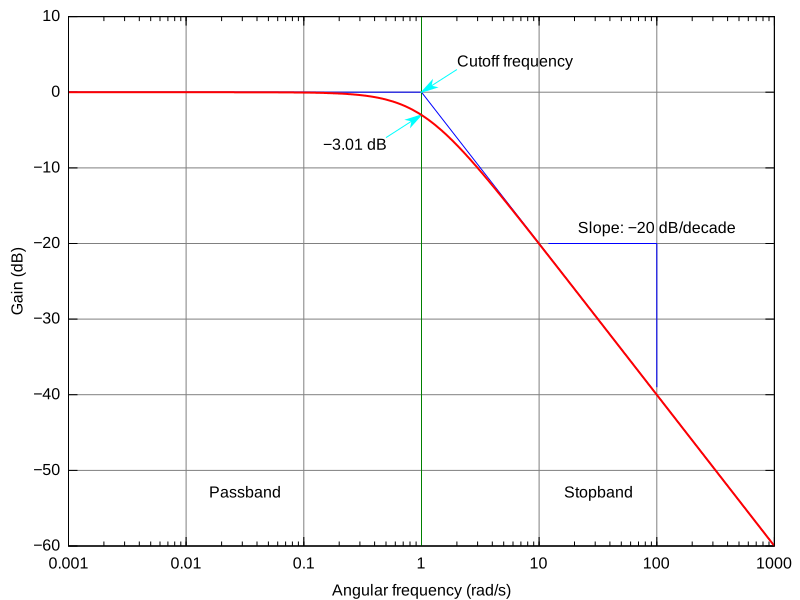
Read the axes first, because half the confusion about filters comes from not doing so. Horizontal is frequency, not time — a point on this graph is a pitch, not a moment. Vertical is how much of that frequency gets through, with 1 meaning untouched and 0 meaning removed entirely.
Three features have names you will meet constantly:
The passband is the flat region on the left where the curve sits near 1. Frequencies here pass essentially unchanged, which is the filter's job.
The cutoff is where the curve has fallen to 1/\sqrt2, about 0.707, which is half the power — since power goes as amplitude squared and 0.707^2 = 0.5. That is the origin of the phrase "the −3 dB point", because 10\log_{10}(0.5) = -3.
The roll-off is the slope after cutoff, and the picture shows the trade the whole chapter turns on: a higher order gives a steeper roll-off, and it costs more computation and more delay. There is no filter with a vertical edge, and the reason is Chapter 4.4's time–frequency trade — a perfectly sharp cut in frequency needs a filter of infinite length in time.
3. IIR filters
y[n]=\sum_kb_kx[n-k]-\sum_ka_ky[n-k]
Feedback gives enormous efficiency. A 4th-order IIR filter can match a 100-tap FIR for sharpness, using 8 multiplications instead of 100.
Design by transformation
Nobody designs IIR filters from scratch. The method is to take a well-understood analog design and convert it, which lets a century of analog filter theory carry over intact.
The starting points are the classical analog responses:
- Butterworth — maximally flat passband, moderate roll-off. The default.
- Chebyshev type I — steeper, with ripple in the passband.
- Chebyshev type II — steeper, with ripple in the stopband.
- Elliptic (Cauer) — steepest possible for a given order, with ripple in both. Also the worst phase behaviour.
- Bessel — gentlest roll-off, but nearly constant group delay. The only analog family that tries to preserve waveform shape.
The trade across that list is monotonic: each step buys sharpness with ripple and with phase distortion. Butterworth when you have no strong reason otherwise; elliptic when you must have the sharpest possible response and do not care about phase; Bessel when waveform shape matters more than filtering.
The bilinear transform
The conversion from s to z:
s=\frac{2}{T}\cdot\frac{1-z^{-1}}{1+z^{-1}}
Why this particular formula: it maps the entire left half of the s-plane into the interior of the unit circle, one-to-one. So a stable analog filter always becomes a stable digital one — no exceptions, no checking required.
The catch is frequency warping. The mapping squeezes the infinite analog frequency axis into the finite range 0 to f_s/2, and the squeezing is non-linear:
\omega_{analog}=\frac{2}{T}\tan\!\left(\frac{\omega_{digital}T}{2}\right)
Low frequencies map almost exactly; high frequencies are compressed increasingly. So a filter designed for a 4 kHz cut-off ends up somewhere lower.
The fix is prewarping: compute where the analog cut-off must be so that after warping it lands where you wanted.
Worked example. Want 4 kHz cut-off at 20 kHz sample rate.
\omega_d = 2\pi\times4000 = 25{,}133\ \text{rad/s}, \qquad T = 5\times10^{-5}\ \text{s}
\omega_a=\frac{2}{5\times10^{-5}}\tan\!\left(\frac{25133\times5\times10^{-5}}{2}\right)=40{,}000\tan(0.6283)
=40{,}000\times0.7265=29{,}060\ \text{rad/s} = 4625\ \text{Hz}
Design the analog filter for 4625 Hz, and after the bilinear transform it lands at exactly 4000 Hz. Skip the prewarping and you get about 3.5 kHz instead — a 12% error, which matters.
4. Implementation: why biquads
A high-order IIR filter written as one long difference equation is a trap.
The problem is coefficient sensitivity. The poles are the roots of the denominator polynomial, and the roots of a high-order polynomial move dramatically when its coefficients are perturbed slightly. Round an eighth-order filter's coefficients to 16 bits and its poles can move outside the unit circle, turning your carefully designed filter into an oscillator.
The universal solution is to factor into second-order sections:
H(z)=\prod_{k}\frac{b_{0k}+b_{1k}z^{-1}+b_{2k}z^{-2}}{1+a_{1k}z^{-1}+a_{2k}z^{-2}}
Each biquad has two poles determined by only two coefficients, and the sensitivity collapses. This is how every audio equaliser, every filter library and every DSP implementation does it, and an 8th-order filter is always shipped as four biquads.
Two more implementation decisions that matter in fixed-point arithmetic:
Section ordering. Put the sections with poles closest to the unit circle — the highest-Q, most resonant ones — where they are least likely to overflow, which usually means last. Pair each high-Q pole with the zero nearest to it, so the section's gain stays as flat as possible.
Scaling. Insert gain factors between sections so the signal uses the available numeric range without overflowing. Getting this wrong produces a filter that works perfectly in floating point and produces bursts of loud noise in fixed point.
5. Filter types beyond low-pass
High-pass from low-pass: substitute z^{-1}\to-z^{-1}, which reflects the response about f_s/4. For an FIR, this amounts to alternating the sign of the coefficients.
Band-pass and band-stop come from frequency transformations that turn each pole into a pair. An N-th order low-pass becomes a 2N-th order band-pass, so a band-pass filter is always twice as expensive as it looks.
Notch — Chapter 4.6 built one from scratch by placing zeros on the unit circle. That geometric method is often faster than any transformation.
All-pass. Unity magnitude at every frequency, but a frequency-dependent phase. Used to correct someone else's phase distortion without touching the magnitude — which is exactly what a phase equaliser in a loudspeaker crossover does.
Comb filter. y[n]=x[n]+\alpha x[n-D] produces peaks or notches spaced f_s/D apart across the whole spectrum. This is the flanger effect in audio, and it is also what an echo sounds like in the frequency domain — which explains why a room with a strong reflection has a "hollow" coloration.
6. Multirate processing
Changing the sample rate, which is needed constantly — 44.1 kHz to 48 kHz, oversampling converters, efficient narrowband filtering.
Decimation — reducing the rate
To reduce by a factor M, keep every M-th sample.
But you must filter first. After decimation the new Nyquist frequency is f_s/2M, and anything above it aliases (Chapter 4.7). So a low-pass filter with cut-off at f_s/2M must be applied before discarding samples.
The clever part: the filter only needs to produce the samples you are keeping. Computing outputs you immediately discard is pure waste, so a polyphase implementation computes only every M-th output, cutting the work by exactly M.
Interpolation — increasing the rate
To increase by L, insert L-1 zeros between samples, then low-pass filter to smooth them out.
Why inserting zeros works, and it is not obvious. Zero-stuffing creates images of the spectrum at multiples of the original sample rate — the same replication as sampling in Chapter 4.7. The low-pass filter removes all but the baseband copy, and what remains is a properly interpolated signal.
The polyphase economy applies here too: most of the filter's multiplications involve the inserted zeros and can simply be skipped.
Arbitrary ratios
Converting 44.1 kHz to 48 kHz needs a ratio of 48000/44100 = 160/147. Interpolate by 160, then decimate by 147, using a single filter at the intermediate rate of 7.056 MHz — implemented polyphase so that rate never actually exists in the computation.
Why this ratio is so awkward goes back to Chapter 4.7's history: 44.1 kHz came from video tape line counts and 48 kHz from video frame rates, and the two standards were never designed to relate to each other. That mismatch has cost the audio industry decades of resampling.
7. Numerical effects in real implementations
Three effects that turn a correct design into a broken product.
Coefficient quantisation — covered in section 4. Use biquads.
Round-off noise. Every multiplication produces more bits than it started with, and truncating them injects noise. In an IIR filter this noise circulates through the feedback loop and is amplified by the filter's own gain. The noise is worst where the filter resonates, which is exactly where you were trying to be precise.
Limit cycles. The nastiest one. A stable IIR filter with zero input can settle into a small self-sustaining oscillation, caused entirely by rounding. The filter is mathematically stable and physically oscillating. In an audio path this is an audible tone at low level that never goes away.
The mitigations: use floating point where you can afford it; use more bits in the accumulator than in the coefficients (24-bit coefficients with a 56-bit accumulator is a classic DSP arrangement); add dither, a tiny random signal, to break up the deterministic rounding that limit cycles depend on. The last one is the same trick as Chapter 3.5's dither, applied for the same reason.
8. Choosing, with numbers
A 60 dB low-pass, transition from 0.2 to 0.25 of Nyquist:
- FIR (Parks-McClellan): about 145 taps. 145 multiply-accumulates per sample. Exactly linear phase. Guaranteed stable. Latency 72 samples.
- IIR (elliptic): 6th order, so 3 biquads, about 15 multiply-accumulates per sample. Ten times cheaper. Non-linear phase, especially near the cut-off. Latency of a few samples. Must check stability and numerical behaviour.
Decide on this question: does the shape of the waveform matter?
If you are filtering audio for listening, phase distortion near the cut-off is largely inaudible and the IIR's tenfold saving is decisive. If you are filtering a data signal where the pulse shape carries the bits, or measuring a transient whose shape is the result, the FIR's linear phase is the whole reason you are filtering at all and the extra computation is simply the price.
And when processing offline, the zero-phase trick of Chapter 4.2 — filter forwards, then backwards — gives an IIR filter perfectly linear phase at the cost of doubling the order. That is the best of both, available only when the whole signal is already in memory.
Filters change a signal. Chapter 5.3 is about measuring one — turning the DFT into an honest picture of what a real, noisy, changing signal contains.
Every formula above, built from scratch
None of the results in this chapter are worth memorising, because each one can be rebuilt in under a minute from something simpler. What follows is that rebuilding, one result at a time, so the formula and the reason for it sit on the same page as the explanation that needed them.
FIR filters
y[n]=\sum_{k=0}^{M}b_kx[n-k], \qquad H(z)=\sum_kb_kz^{-k}
Impulse response = the coefficient list, exactly.
Linear phase condition: b_k=b_{M-k} (symmetric) or b_k=-b_{M-k} (antisymmetric).
\text{group delay}=\frac{M}{2}\ \text{samples, at every frequency}
Windowed design. Ideal low-pass impulse response:
h_{ideal}[n]=\frac{\sin(\omega_cn)}{\pi n}, \qquad h_{ideal}[0]=\frac{\omega_c}{\pi}
Where it comes from: the inverse Fourier transform of a rectangle is a sinc (Chapter 4.4). Then truncate to M+1 terms, shift to make it causal, and multiply by a window.
b_k=h_{ideal}\!\left[k-\frac M2\right]\cdot w[k]
Kaiser's order estimate:
M\approx\frac{A-8}{2.285\,\Delta\omega}
A = stopband attenuation in dB, \Delta\omega = transition width in radians per sample.
Read it: taps grow linearly with required attenuation and inversely with transition width. Both are expensive and neither can be avoided.
Rule of thumb for windowed design: M\approx4/(\Delta f/f_s) for a Hann window.
IIR filters
y[n]=\sum_{k=0}^{M}b_kx[n-k]-\sum_{k=1}^{N}a_ky[n-k]
H(z)=\frac{\sum b_kz^{-k}}{1+\sum a_kz^{-k}}
Stable if and only if every pole is inside the unit circle.
Bilinear transform:
s=\frac{2}{T}\cdot\frac{1-z^{-1}}{1+z^{-1}}
Why this one: it maps the entire left half s-plane one-to-one into the unit disc, so a stable analog design always becomes a stable digital one.
Frequency warping:
\omega_{analog}=\frac2T\tan\!\left(\frac{\omega_{digital}T}{2}\right)
Prewarping: compute the analog design frequency from this equation so that after transformation it lands where you wanted it.
Butterworth magnitude:
|H(j\omega)|^2=\frac{1}{1+(\omega/\omega_c)^{2n}}
Maximally flat: the first 2n-1 derivatives at \omega=0 are zero, which is what "maximally flat" means precisely.
Roll-off: 20n dB per decade, or 6n dB per octave.
Chebyshev type I:
|H(j\omega)|^2=\frac{1}{1+\varepsilon^2T_n^2(\omega/\omega_c)}
with T_n the Chebyshev polynomial. Passband ripple =10\log_{10}(1+\varepsilon^2) dB.
Biquad form:
H(z)=\frac{b_0+b_1z^{-1}+b_2z^{-2}}{1+a_1z^{-1}+a_2z^{-2}}
Always factor into biquads above second order. A high-order polynomial's roots move dramatically under coefficient rounding; a second-order section's two poles depend on only two coefficients.
Peaking equaliser (analog prototype, before the bilinear transform):
H(s)=\frac{s^2+\frac{A\omega_0}{Q}s+\omega_0^2}{s^2+\frac{\omega_0}{AQ}s+\omega_0^2}, \qquad A=10^{G/40}
Q=\frac{f_0}{\text{bandwidth}}
Multirate
Decimation by M: low-pass at f_s/2M first, then keep every M-th sample. Polyphase implementation computes only the retained outputs, cutting work by M.
Interpolation by L: insert L-1 zeros, then low-pass at f_s/2L with gain L. Polyphase skips the multiplications involving inserted zeros.
Rational resampling by L/M: interpolate by L, filter once at the intermediate rate, decimate by M.
\frac{48000}{44100}=\frac{160}{147}
Noise shaping and oversampling gain:
\Delta\text{SNR}=10\log_{10}(\text{OSR}) \ \text{dB}
What the next chapter fixes
Every spectrum so far has come from a clean, complete stretch of signal. Real measurements are taken from a finite window of something that did not start when you started looking, and that alone puts energy into the answer that was never in the signal. Chapter 5.3 explains where that leakage comes from and what window functions do about it.