Appearance
6.6 — PID Controllers
Somewhere between 90 and 95% of all industrial control loops are PID. Not because it is optimal — it is not — but because it needs no model of the plant, it has three parameters a person can understand, and it works.
Nicolas Minorsky derived it in 1922 from watching how a helmsman steers a ship, and the observation is worth carrying: a good helmsman does not simply turn the wheel in proportion to how far off course the ship is. He also turns further if the ship has been off course for a while, and he eases off if the ship is already swinging back quickly. Those three behaviours are exactly proportional, integral and derivative.
1. The three terms
u(t)=K_pe(t)+K_i\int_0^te(\tau)d\tau+K_d\frac{de(t)}{dt}
C(s)=K_p+\frac{K_i}{s}+K_ds
In words, each term answers a different question about the error:
- Proportional — how big is the error right now?
- Integral — how long has it been wrong?
- Derivative — which way is it heading?
Proportional
u=K_pe
The obvious response: bigger error, bigger correction.
What raising K_p does: faster response, smaller steady-state error, more overshoot, less stability margin.
What it cannot do: eliminate steady-state error. Chapter 6.2 showed why. For a type 0 plant:
e_{ss}=\frac{1}{1+K_pG(0)}
Zero error would need zero output from the controller, but zero output means nothing is driving the plant. A heater holding a room above ambient must keep supplying power, and if the error is zero then K_pe = 0 and the power is zero. The error is not a flaw in the tuning; it is structurally necessary.
That permanent offset has a traditional name from process control: droop.
Integral
u=K_i\int e\,dt
The integral accumulates. As long as any error persists, the integral keeps growing and the output keeps rising. It only stops changing when the error is exactly zero.
That is the whole mechanism, and it is worth stating as a principle: an integrator's output can be non-zero while its input is zero, which is precisely what a steady-state offset requires.
What it costs. An integrator contributes -90° of phase at every frequency, which comes straight out of the phase margin. More integral action always means less stability, and this is the fundamental trade of PID tuning.
Integral windup — the failure everyone meets. Suppose the plant saturates: the valve is fully open, the heater is at maximum, the motor is at full voltage. The error persists because the plant physically cannot do more. The integral keeps accumulating anyway, sometimes to enormous values.
When the setpoint is finally reached, the accumulated integral is still driving the output hard, and the system overshoots massively and takes a long time to recover while the integral unwinds.
Three standard fixes:
- Clamping. Stop integrating whenever the output is saturated.
- Back-calculation. Feed the difference between the requested and actual output back into the integrator to unwind it at a controlled rate.
- Conditional integration. Only integrate when the error is small enough that the plant is not saturated.
Anti-windup is not an optional refinement. Any loop that can saturate — which is every real loop — needs it, and its absence is one of the most common causes of a controller that behaves well in simulation and badly on the machine.
Derivative
u=K_d\frac{de}{dt}
Responds to the rate of change, not the magnitude. If the error is large but shrinking fast, the derivative term reduces the output — it anticipates the approach and eases off before overshooting.
What it buys: damping. It adds a zero at s=-K_p/K_d, and Chapter 6.4 showed that a zero pulls the root locus leftward. More stability margin and less overshoot, so you can then raise K_p further than you otherwise could.
What it costs, and this is why derivative is often left out entirely:
Noise amplification. Differentiation multiplies each frequency component by \omega, so high-frequency noise is amplified in proportion to its frequency. A measurement with 1% noise at 100 times the loop bandwidth becomes 100% noise after differentiation.
The fix is always a filtered derivative:
\frac{K_ds}{1+sT_f}, \qquad T_f=\frac{K_d}{NK_p}, \quad N=8\text{ to }20
Read the structure: it differentiates at low frequency and levels off to a constant gain of K_d/T_f above the filter corner, so noise is amplified by at most N rather than without limit. Every real derivative implementation has this filter, and a "pure" K_ds is a textbook object that nobody builds.
Derivative kick. If the setpoint changes as a step, its derivative is an impulse, and the controller output spikes enormously for one sample.
The fix is elegant and universal: differentiate the measurement rather than the error.
u=K_pe+K_i\int e\,dt-K_d\frac{dy}{dt}
Note the minus sign — the measurement's derivative has the opposite sign to the error's. Since the measurement cannot jump when the setpoint does (the plant has inertia), there is no kick. The behaviour for disturbances is unchanged, and this is what every commercial controller does.
The same reasoning applied to the proportional term gives setpoint weighting: use \beta r - y instead of r - y in the proportional term, with \beta between 0 and 1, to soften the response to setpoint changes without affecting disturbance rejection.
Watching the three terms take effect
The three terms are easier to believe once you have seen each one change the same response.
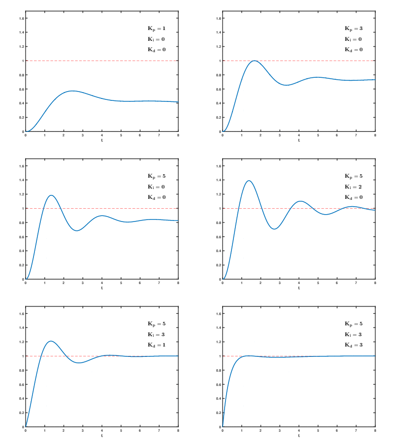
Watch each term separately, because the animation shows exactly what the equations in section 1 predict.
Raising the proportional gain K_p makes the response faster and increases the overshoot, and past a point it will not settle at all. It also never quite reaches the target, because a proportional controller needs a non-zero error to produce any output — that leftover gap is the steady-state error of Chapter 6.3.
Raising the integral gain K_i drags the curve onto the target and holds it there, because the integral keeps accumulating for as long as any error remains and only stops growing when the error is exactly zero. That is the term that kills steady-state error, and it is the reason almost no real controller is proportional-only. It costs you extra overshoot and a slower settle, because the accumulated total has to be unwound again.
Raising the derivative gain K_d damps the ringing, because the derivative responds to how fast the error is changing and therefore pushes back hardest while the output is racing towards the target. It is the brake. It also amplifies measurement noise badly, since differentiating a noisy signal magnifies the noise, which is why many industrial loops are run as PI with no D at all.
2. Tuning
Ziegler-Nichols, and its honest assessment
John Ziegler and Nathaniel Nichols published two methods in 1942, and they remain the best-known starting points.
The ultimate gain method:
- Set K_i = K_d = 0.
- Raise K_p until the loop oscillates with a steady amplitude. Call that gain K_u and the oscillation period T_u.
- Apply the table.
| Controller | K_p | T_i | T_d |
|---|---|---|---|
| P | 0.5K_u | — | — |
| PI | 0.45K_u | T_u/1.2 | — |
| PID | 0.6K_u | T_u/2 | T_u/8 |
where K_i = K_p/T_i and K_d = K_pT_d.
Notice what K_u and T_u actually are. K_u is the critical gain that Routh-Hurwitz computes (Chapter 6.4), and T_u is the period of the imaginary-axis oscillation. The method is an experimental measurement of the stability boundary, which is why it needs no model.
The honest assessment. Ziegler-Nichols tuning is aggressive — it typically gives a quarter-amplitude decay, meaning each overshoot is a quarter of the last, which corresponds to about 50% overshoot and \zeta \approx 0.22. That is unacceptably oscillatory for most modern applications, and it was chosen in 1942 for fast disturbance rejection in process plants where overshoot mattered less.
Use it as a starting point and then reduce K_p by a factor of 2, which typically gives 10 to 20% overshoot.
And the method itself is risky: deliberately driving a plant to sustained oscillation is not acceptable on most real equipment. Which is why the second method exists.
The step response method uses an open-loop step test. Measure the dead time L (how long before anything happens) and the slope R of the steepest part of the rise. Then:
| Controller | K_p | T_i | T_d |
|---|---|---|---|
| P | 1/RL | — | — |
| PI | 0.9/RL | 3L | — |
| PID | 1.2/RL | 2L | 0.5L |
Read the structure: everything is set by the ratio of dead time to time constant, which is the single number that determines how hard a plant is to control. A plant with dead time comparable to its time constant is genuinely difficult, for exactly the phase-lag reason of Chapter 6.5.
Manual tuning
The procedure that most engineers actually use, and it works:
- Set K_i and K_d to zero. Raise K_p until the response is fast with modest overshoot, then back off about 30%.
- Add K_i, increasing until the steady-state error disappears quickly enough. Too much and it oscillates slowly — a lazy, wandering oscillation is the signature of excessive integral.
- Add K_d if needed, to reduce overshoot. Too much and the output becomes jittery — visible noise on the actuator is the signature of excessive derivative.
- Iterate, and test the disturbance response separately from the setpoint response.
Reading the symptom is the skill:
| Symptom | Likely cause |
|---|---|
| Fast oscillation | K_p too high |
| Slow, wandering oscillation | K_i too high |
| Jittery, noisy actuator | K_d too high |
| Never quite reaches setpoint | K_i too low or absent |
| Sluggish | K_p too low |
| Huge overshoot after saturation | windup, no anti-windup |
Lambda tuning
For process control, a more predictable method. Choose a desired closed-loop time constant \lambda, then for a first-order-plus-dead-time plant with gain K, time constant \tau and dead time L:
K_p=\frac{\tau}{K(\lambda+L)}, \qquad T_i=\tau
One parameter, \lambda, and it directly means "how fast do you want this to be". Setting \lambda = \tau gives a conservative, robust loop; \lambda = \tau/3 gives an aggressive one. This is far easier to explain to an operator than three gains, and it is why process industries have largely moved to it.
3. What PID cannot do
Worth knowing, because it saves you from tuning something that cannot be tuned.
Long dead time. When the dead time exceeds roughly the plant's time constant, PID performance collapses — the loop must be detuned so far that it barely helps. The answer is a Smith predictor, which uses a model of the plant to predict what the output will be after the delay and controls that prediction instead, effectively removing the delay from the loop. It requires an accurate model, which PID does not, and that is the trade.
Non-minimum phase plants. The right-half-plane zero of Chapter 6.2 places a hard bandwidth limit that no PID tuning escapes.
Multiple interacting loops. Two PID loops controlling variables that affect each other will fight. Detuning both is the usual crude answer; a proper multivariable controller is the right one.
Hard constraints. PID has no concept of "the valve cannot exceed 80% because of a safety rule". Model predictive control optimises over a horizon with constraints built in, which is why it dominates in refineries and chemical plants.
Highly nonlinear plants. A single set of gains cannot suit a plant whose behaviour changes with operating point. Gain scheduling — a table of gains indexed by operating condition — is the standard practical answer, and it is what every aircraft flight control system does with airspeed and altitude.
4. Implementing PID in software
The discrete form, using the backward difference for the derivative and a rectangular sum for the integral:
u[n]=K_pe[n]+K_iT_s\sum_{k=0}^{n}e[k]+\frac{K_d}{T_s}\left(e[n]-e[n-1]\right)
The velocity form is usually better, computing the change in output rather than the output itself:
\Delta u[n]=K_p(e[n]-e[n-1])+K_iT_se[n]+\frac{K_d}{T_s}(e[n]-2e[n-1]+e[n-2])
u[n]=u[n-1]+\Delta u[n]
Two real advantages. There is no explicit integral accumulator, so windup is handled simply by clamping u — the accumulated history lives in u[n-1], which is already limited. And switching between manual and automatic control is bumpless, because the controller starts from wherever the output already is rather than from a stale integral.
The implementation checklist
Sample rate. 10 to 20 times the closed-loop bandwidth minimum, and Chapter 6.4's analysis argued for 20 to 40. The half-sample delay costs phase margin directly.
Sample at a strictly constant rate. Jitter in the sampling interval is jitter in the effective K_i and K_d, since both scale with T_s. Use a timer interrupt, never a delay loop in the main program.
Output limiting to the actuator's real range, with anti-windup.
Rate limiting where a sudden actuator movement would damage something.
Deadband — do nothing while the error is under a threshold — where actuator wear matters. A valve that adjusts continuously wears out; one that adjusts only when the error exceeds 0.5% lasts years longer.
Filter the measurement, but remember Chapter 6.4's warning: the filter's pole eats phase margin. A filter corner at ten times the crossover frequency costs about 6° of margin, which is usually acceptable; at three times it costs 18°, which usually is not.
Bumpless transfer when switching modes or changing gains, so the output does not jump.
5. Three worked applications
A temperature controller
Plant: an oven, first order with a 200 s time constant and 20 s dead time, gain 2 °C per percent of heater power.
Lambda tuning with \lambda = 100 s (aggressive but reasonable):
K_p=\frac{200}{2(100+20)}=0.83\ \%/°\text{C}, \qquad T_i=200\ \text{s}, \qquad K_i=\frac{0.83}{200}=0.00417
No derivative — a thermal system's measurement is noisy and its dynamics are slow, so derivative buys little and costs noise.
Sample rate: the closed-loop time constant is 100 s, so sampling every 1 s is 100 times faster than needed. 1 s is fine and even 5 s would work, which is why oven controllers are undemanding.
Anti-windup is essential, because the heater saturates at 100% during every warm-up from cold, and without clamping the first approach to setpoint would overshoot by tens of degrees.
A motor speed controller
Plant: first order, 50 ms time constant, gain 100 rpm per volt.
Target: settling time 100 ms, so a closed-loop time constant of 25 ms.
K_p=\frac{\tau}{K\lambda}=\frac{0.05}{100\times0.025}=0.02\ \text{V/rpm}, \qquad T_i=0.05\ \text{s}, \qquad K_i=0.4
Sample rate: closed-loop bandwidth is 1/(2\pi\times0.025)=6.4 Hz, so sample at 20 to 40 times that — 200 Hz, giving a 5 ms period. In practice motor loops run at 1 to 10 kHz because the current loop underneath needs it.
Derivative: usually omitted for speed loops, because the speed measurement from an encoder is already a difference and therefore noisy.
A quadcopter attitude loop
Cascaded loops, which is the standard architecture for anything with position and rate:
- Inner loop: angular rate, running at 1 to 8 kHz, PID with strong derivative.
- Outer loop: angle, running at 250 to 500 Hz, mostly proportional.
Why cascade rather than one loop? The inner loop is fast and handles disturbances — wind, propeller imbalance — before they can affect the angle at all. The outer loop then sees a well-behaved, nearly ideal rate-controlled plant rather than the raw dynamics.
The rule for any cascade: the inner loop must be at least five times faster than the outer, or they interact and both must be detuned.
Practical realities. The gyroscope's noise makes derivative action difficult, so it is heavily filtered. Propeller vibration appears as a strong peak in the gyro signal, and a notch filter (Chapter 4.6) at the propeller frequency is standard. And the loop must be tuned per airframe, because the inertia and motor response change with size and weight — which is why every flight controller ships with a tuning procedure rather than fixed gains.
PID uses one input and one output and no model. Chapter 6.7 introduces the framework that handles many of each, and uses the model explicitly.
Every formula above, built from scratch
None of the results in this chapter are worth memorising, because each one can be rebuilt in under a minute from something simpler. What follows is that rebuilding, one result at a time, so the formula and the reason for it sit on the same page as the explanation that needed them.
PID
C(s)=K_p+\frac{K_i}{s}+K_ds=K_p\left(1+\frac{1}{T_is}+T_ds\right)
K_i=\frac{K_p}{T_i}, \qquad K_d=K_pT_d
Filtered derivative (compulsory in practice):
\frac{K_ds}{1+sT_f}, \qquad T_f=\frac{K_d}{NK_p}, \quad N=8\text{ to }20
Derivative on measurement, to avoid setpoint kick:
u=K_pe+K_i\int e\,dt-K_d\frac{dy}{dt}
Ziegler-Nichols, ultimate gain method
| Controller | K_p | T_i | T_d |
|---|---|---|---|
| P | 0.5K_u | — | — |
| PI | 0.45K_u | T_u/1.2 | — |
| PID | 0.6K_u | T_u/2 | T_u/8 |
Gives roughly quarter-amplitude decay, which is \zeta\approx0.22 and about 50% overshoot. Halve K_p for a usable loop.
Ziegler-Nichols, step response method
With dead time L and slope R:
| Controller | K_p | T_i | T_d |
|---|---|---|---|
| P | 1/RL | — | — |
| PI | 0.9/RL | 3L | — |
| PID | 1.2/RL | 2L | 0.5L |
Lambda tuning
For a first-order-plus-dead-time plant with gain K, time constant \tau, dead time L, and desired closed-loop time constant \lambda:
K_p=\frac{\tau}{K(\lambda+L)}, \qquad T_i=\tau
\lambda=\tau is conservative; \lambda=\tau/3 is aggressive.
Discrete implementation
Position form:
u[n]=K_pe[n]+K_iT_s\sum_{k\le n}e[k]+\frac{K_d}{T_s}(e[n]-e[n-1])
Velocity form (preferred — inherent anti-windup and bumpless transfer):
\Delta u[n]=K_p(e[n]-e[n-1])+K_iT_se[n]+\frac{K_d}{T_s}(e[n]-2e[n-1]+e[n-2])
Sample rate: 20 to 40 times the closed-loop bandwidth. The half-sample delay T_s/2 contributes phase lag \omega T_s/2, which comes straight out of the phase margin.
What the next chapter fixes
PID handles one input driving one output. A real aircraft, robot arm or chemical plant has many of each, all interacting, and a transfer function cannot express that without becoming a matrix of transfer functions. Chapter 6.7 changes representation entirely, describing the system by its internal state instead, which handles any number of inputs and outputs with the same equations.