Appearance
4.4 — Fourier Series and the Fourier Transform
Play a note on a violin and a note on a flute at the same pitch. They sound completely different, and yet both are periodic at the same frequency. The difference is entirely in what else is in there — the harmonics, and how much of each.
Joseph Fourier's claim, made in 1807 in a paper about heat flow in metal bars, was far stronger than that: any periodic signal, however jagged, is a sum of sines. A square wave with its perfect vertical edges is a sum of smooth curves. Lagrange, on the review committee, refused to believe it and blocked publication for fifteen years.
Fourier was right, with conditions, and the result is the most useful idea in engineering.
This chapter is the engineering face of Volume II Chapter 9.2, and it depends on exactly one fact from Chapter 4.1: that sines at different frequencies are orthogonal, so measuring one does not disturb another. Every formula below is that fact used as a measuring instrument.
The letters this chapter uses, said out loud
Fourier analysis is where the symbols get dense, and every one of them is standing in for something concrete.
\omega — "omega", angular frequency, in radians per second. It relates to ordinary frequency by \omega = 2\pi f, and the 2\pi is there because one full cycle is 2\pi radians of angle. Engineers write f in hertz on datasheets and \omega in the mathematics, and forgetting to convert between them is the most common numerical error in this Part.
\omega_0 — "omega nought", the fundamental frequency: the frequency of the slowest sine in the series, set by the signal's own repetition period as \omega_0 = 2\pi/T. Every other component is a whole-number multiple of it.
n — the harmonic number, a plain integer. The n-th harmonic has frequency n\omega_0. It is a counter, not a measured quantity.
a_n and b_n — how much cosine and how much sine the signal contains at the n-th harmonic. Both have the same units as the signal itself. The letters are simply the first two of the alphabet, from Fourier's own 1822 notation.
c_n — the same information in complex form, one number holding both an amount and a phase shift. Section 3 shows why one complex number is easier to work with than two real ones.
j — the square root of -1. Mathematics writes i; electrical engineering writes j because i was already taken by current, and that collision is why the whole field uses the odd-looking letter. Volume II Chapter 2.5 covers what it means.
X(\omega) — "big X of omega", the spectrum: a function saying how much of every frequency the signal contains. Capital letters are used for frequency-domain quantities and lower case for time-domain ones throughout this Part, so x(t) and X(\omega) are the same signal in its two descriptions.
T and f — period in seconds and frequency in hertz, reciprocals of each other. T is from time; the hertz is named after Heinrich Hertz, who generated and detected radio waves in 1887 and so proved Maxwell right.
1. The Fourier series
A periodic signal x(t) with period T and fundamental frequency \omega_0 = 2\pi/T can be written
x(t)=a_0+\sum_{n=1}^{\infty}\left[a_n\cos(n\omega_0t)+b_n\sin(n\omega_0t)\right]
Read aloud: "x of t equals a-nought plus the sum from n equals one to infinity of a-n cosine n omega-nought t plus b-n sine n omega-nought t."
In words: a constant, plus a sine and cosine at the fundamental, plus a sine and cosine at twice the fundamental, and so on forever. The n-th term is the n-th harmonic.
Finding the coefficients
This is where Chapter 4.1's orthogonality earns its place. Because
\int_0^T\cos(m\omega_0t)\cos(n\omega_0t)\,dt = \begin{cases}T/2 & m=n\\0 & m\ne n\end{cases}
multiplying the whole series by \cos(m\omega_0t) and integrating over one period kills every term except the one you multiplied by. That single term survives with a factor of T/2.
\boxed{a_n = \frac{2}{T}\int_0^Tx(t)\cos(n\omega_0t)\,dt, \qquad b_n=\frac{2}{T}\int_0^Tx(t)\sin(n\omega_0t)\,dt}
a_0 = \frac{1}{T}\int_0^Tx(t)\,dt
Note that a_0 has 1/T and not 2/T — it is the plain average, the DC component, and it comes out of the same derivation with the cosine replaced by 1.
The physical reading of the coefficient formula: to find how much of frequency n is present, multiply by frequency n and average. If the signal contains that frequency, the product is positive on average; if not, it averages to zero. It is a correlation, exactly as in Chapter 4.3 — you are correlating the signal against each candidate frequency in turn.
The exponential form
Combining sine and cosine with Euler's formula gives the form actually used in practice:
x(t)=\sum_{n=-\infty}^{\infty}c_ne^{jn\omega_0t}, \qquad c_n=\frac{1}{T}\int_0^Tx(t)e^{-jn\omega_0t}\,dt
One formula instead of three, at the cost of negative frequencies, which are a bookkeeping device rather than a physical claim: c_n and c_{-n} are complex conjugates for a real signal, and they pair up to give a real cosine.
|c_n|=\tfrac12\sqrt{a_n^2+b_n^2}, \qquad \angle c_n = -\arctan\frac{b_n}{a_n}
2. Worked example — the square wave
Before the algebra, watch it happen. A square wave has sharp vertical edges and flat tops, and sine waves have neither. The claim that adding up enough sines produces one sounds false until you see it being built.
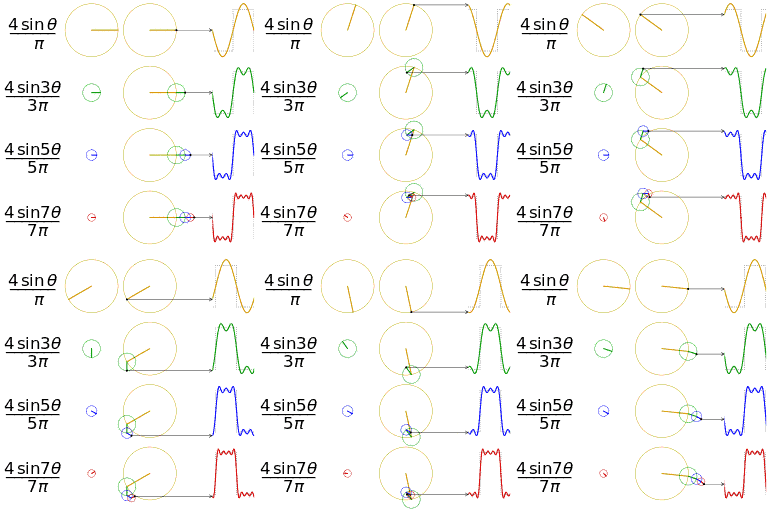
Read the picture with the formula you are about to derive in mind, because everything in that formula is visible in it. The circles turn at 1\times, 3\times, 5\times the fundamental rate — only odd multiples, and the derivation below is going to show every even one coming out as exactly zero. Their radii fall as 1, \tfrac13, \tfrac15 — that 1/n shrinkage is the 2/\pi n that appears in the answer. And the edges are the last thing to sharpen: with three circles the corners are rounded, with twenty they are crisp, and a genuinely vertical edge needs infinitely many. That is not an artefact of the drawing. It is why a square pulse sent down a channel of limited bandwidth arrives with rounded corners, which Chapter 7.1 turns into a bit-rate limit.
Now the algebra, which says the same thing in symbols.
A square wave of amplitude 1, period T, odd (so +1 for the first half, -1 for the second).
Symmetry does most of the work. The signal is odd, so every a_n is zero — an odd signal cannot contain any cosine, which is even. Only sines survive.
b_n=\frac{2}{T}\int_0^Tx(t)\sin(n\omega_0t)\,dt = \frac{2}{T}\left[\int_0^{T/2}\sin(n\omega_0t)dt-\int_{T/2}^{T}\sin(n\omega_0t)dt\right]
Both integrals are the same by symmetry, so:
=\frac{4}{T}\int_0^{T/2}\sin(n\omega_0t)\,dt = \frac{4}{T}\left[\frac{-\cos(n\omega_0t)}{n\omega_0}\right]_0^{T/2}
With \omega_0=2\pi/T, the upper limit gives n\omega_0 T/2 = n\pi:
=\frac{4}{Tn\omega_0}\left[1-\cos(n\pi)\right] = \frac{2}{\pi n}\left[1-(-1)^n\right]
For even n, (-1)^n = 1 and the bracket is zero. For odd n it is 2:
b_n = \frac{4}{\pi n} \quad(n \text{ odd}), \qquad 0 \quad(n \text{ even})
x(t)=\frac{4}{\pi}\left[\sin\omega_0t+\frac13\sin3\omega_0t+\frac15\sin5\omega_0t+\frac17\sin7\omega_0t+\cdots\right]
Three things to take from this result.
Only odd harmonics. That comes from half-wave symmetry — the second half of the period is the negative of the first. Any signal with that symmetry has only odd harmonics, and it is why a square wave and a triangle wave both have that character while a sawtooth, which lacks the symmetry, has all harmonics.
Amplitudes fall as 1/n. Slowly. The 99th harmonic is still 1% of the fundamental. Sharp corners need high frequencies, and that is the general rule: the faster a signal changes, the further its spectrum extends.
A useful reality check. At \omega_0t=\pi/2 the series gives \frac4\pi(1-\frac13+\frac15-\frac17+\cdots), and it should equal 1. So the bracket must equal \pi/4 — which is the Leibniz series for \pi, arrived at from a completely different direction.
Gibbs phenomenon
Truncate the series at any finite number of terms and something stubborn happens: near each discontinuity the partial sum overshoots by about 9% of the jump height, and adding more terms does not reduce the overshoot. It only makes the overshoot narrower, squeezing it closer to the edge.
Why it never goes away: the overshoot's area shrinks towards zero, so the series converges in an energy sense, but its height converges to about 1.089 times the jump. Convergence in energy does not imply convergence at every point, and a discontinuity is exactly where the difference shows.
Josiah Willard Gibbs explained it in 1899, after Albert Michelson built a mechanical harmonic analyser and found the ripple, assumed his machine was faulty, and wrote to Nature about it.
Practically: every filter that sharply truncates a spectrum produces this ripple. It is the reason digital filter design uses windows instead of hard cut-offs (Chapter 5.2), and it is visible as the ringing halo around sharp edges in an over-compressed JPEG.
3. From series to transform
The Fourier series needs a periodic signal. What about a single pulse, which never repeats?
The trick is to let the period go to infinity. Take a pulse and repeat it every T seconds; the series has harmonics spaced \omega_0=2\pi/T apart. Now stretch T. The harmonics crowd closer. As T\to\infty the spacing goes to zero and the discrete line spectrum becomes a continuous one.
\boxed{X(\omega)=\int_{-\infty}^{\infty}x(t)e^{-j\omega t}\,dt}
\boxed{x(t)=\frac{1}{2\pi}\int_{-\infty}^{\infty}X(\omega)e^{j\omega t}\,d\omega}
The first is the Fourier transform, the second the inverse. Read the forward one: "X of omega equals the integral over all time of x of t times e to the minus j omega t, dee t."
The physical meaning is unchanged from the series. e^{-j\omega t} is a probe at frequency \omega; multiplying and integrating measures how much of that frequency the signal contains. The only difference is that every frequency is now available, not just multiples of a fundamental.
Using f in hertz instead of \omega in radians per second removes the 2\pi from the inverse and makes the pair symmetric:
X(f)=\int x(t)e^{-j2\pi ft}dt, \qquad x(t)=\int X(f)e^{j2\pi ft}df
Both conventions are in use. Check which one a formula assumes before trusting a factor of 2\pi.
The two views of the same signal, side by side
The transform is easier to trust once you have watched a signal and its spectrum change together. The picture below shows exactly that: the same waveform drawn in time along one axis and in frequency along the other.

Three things in that picture are worth naming, because each is a result you will use for the rest of the volume.
Nothing is lost going either way. The transform is invertible, so the spectrum is not a summary of the signal — it is the signal, written in a different alphabet. That is why an equaliser can alter one frequency band and hand back a perfectly ordinary sound.
A pure sine gives a single spike. One frequency in, one line out. Anything more complicated than a sine is a signal containing more than one frequency, and the number of spikes is a direct count of how many.
Sharp features in time need wide bandwidth in frequency, and vice versa. Squeeze the pulse and the spectrum spreads; stretch it and the spectrum narrows. Section 5 makes that trade exact, and it is the single most consequential fact in the whole of communication engineering.
4. The transform pairs worth knowing by heart
Rectangle and sinc
For a pulse of height 1 from -T/2 to T/2:
X(\omega)=\int_{-T/2}^{T/2}e^{-j\omega t}dt=\left[\frac{e^{-j\omega t}}{-j\omega}\right]_{-T/2}^{T/2} = \frac{e^{j\omega T/2}-e^{-j\omega T/2}}{j\omega}
The numerator is 2j\sin(\omega T/2) by Euler, so:
X(\omega)=\frac{2\sin(\omega T/2)}{\omega}=T\,\text{sinc}\!\left(\frac{\omega T}{2\pi}\right)
A rectangle in time is a sinc in frequency. And by the symmetry of the transform, a rectangle in frequency — an ideal brick-wall filter — is a sinc in time. That is Chapter 4.7's whole story about reconstruction, and the reason perfect filters cannot be built.
The scaling matters as much as the shape. The first zero of the sinc is at \omega = 2\pi/T, so:
\boxed{\text{narrow pulse} \Longleftrightarrow \text{wide spectrum}}
Halve the pulse width and the spectrum doubles in width. This is the time-bandwidth trade, and it is not negotiable. It is why a radar wanting fine range resolution needs a wide bandwidth, why a fast digital edge radiates across the spectrum, and why a photograph cannot be simultaneously sharp and free of noise.
Taken to its limit, an impulse — infinitely narrow — has a transform that is flat across all frequencies:
\delta(t) \;\longleftrightarrow\; 1
This is why the impulse response tells you everything. An impulse contains every frequency equally, so the response to it reveals what the system does at every frequency at once. It is also why tapping something is a legitimate way to find its resonances.
The others
| Time | Frequency |
|---|---|
| \delta(t) | 1 |
| 1 | 2\pi\delta(\omega) |
| e^{-at}u(t) | \dfrac{1}{a+j\omega} |
| \cos\omega_0t | \pi[\delta(\omega-\omega_0)+\delta(\omega+\omega_0)] |
| e^{-t^2/2} | \sqrt{2\pi}\,e^{-\omega^2/2} |
The last row is remarkable: a Gaussian transforms into a Gaussian. It is the only shape that keeps its form, and it is also the shape that minimises the time-bandwidth product — the closest anything gets to being localised in both domains at once. That fact underlies the uncertainty principle in quantum mechanics, which is the same mathematics with position and momentum in place of time and frequency.
5. The properties, and the one that matters most
Linearity. ax_1+bx_2 \leftrightarrow aX_1+bX_2.
Time shift. x(t-t_0) \leftrightarrow X(\omega)e^{-j\omega t_0}.
A delay changes only the phase, never the magnitude. The phase shift is proportional to frequency, with slope -t_0. That is why group delay, defined as -d\phi/d\omega, measures the actual delay a system imposes, and why a system with non-linear phase smears a pulse — different frequencies arrive at different times.
Frequency shift (modulation). x(t)e^{j\omega_ct} \leftrightarrow X(\omega-\omega_c).
Multiplying by a complex exponential shifts the whole spectrum. In real terms:
x(t)\cos(\omega_ct) \;\longleftrightarrow\; \tfrac12X(\omega-\omega_c)+\tfrac12X(\omega+\omega_c)
This is the entire theory of radio in one line. A 5 kHz audio signal multiplied by a 1 MHz carrier appears as two copies of the audio spectrum, centred at ±1 MHz. Chapter 7.2 does nothing but exploit this.
Scaling. x(at) \leftrightarrow \frac{1}{|a|}X(\omega/a). Compress in time, expand in frequency — the trade of section 4 stated generally.
The convolution theorem
\boxed{x(t)*h(t) \;\longleftrightarrow\; X(\omega)H(\omega)}
x(t)h(t) \;\longleftrightarrow\; \frac{1}{2\pi}X(\omega)*H(\omega)
Convolution in one domain is multiplication in the other. This is the reason for everything.
Proof sketch, which is short enough to be worth seeing. Take the transform of the convolution:
\int\left[\int x(\tau)h(t-\tau)d\tau\right]e^{-j\omega t}dt
Swap the order of integration and substitute u = t-\tau, so t = u+\tau and e^{-j\omega t}=e^{-j\omega\tau}e^{-j\omega u}:
=\int x(\tau)e^{-j\omega\tau}\left[\int h(u)e^{-j\omega u}du\right]d\tau = X(\omega)H(\omega)
The inner bracket is H(\omega), independent of \tau, so it comes out — and what is left is X(\omega).
Every consequence in this volume flows from this. A filter's effect becomes multiplication by its frequency response. Cascaded systems multiply. Filter design becomes shaping a curve. And Chapter 5.1's FFT-based fast convolution exists precisely because multiplying is cheaper than convolving.
Parseval's theorem
\int_{-\infty}^{\infty}|x(t)|^2dt = \frac{1}{2\pi}\int_{-\infty}^{\infty}|X(\omega)|^2d\omega
Total energy is the same whether you count it in time or in frequency. The transform redistributes energy across frequency without creating or destroying any. |X(\omega)|^2 is therefore called the energy spectral density — energy per unit frequency — and it is what a spectrum analyser plots.
6. Magnitude and phase, and why phase is undervalued
X(\omega) is complex, so it carries two pieces of information at every frequency:
|X(\omega)| = \text{how much of this frequency}, \qquad \angle X(\omega) = \text{where its peaks sit in time}
Almost every spectrum you have seen plotted shows only the magnitude, and this creates a false impression that phase is a detail.
Here is the experiment that corrects it. Take two photographs. Transform both. Build a new image from image A's magnitude and image B's phase, and transform back.
You see image B. Recognisably, unmistakably. The phase carries the structure — where the edges are, where the objects are — while the magnitude carries only the texture statistics.
The same holds for audio in a weaker form. Randomise the phases of a recording while keeping magnitudes and you get noise with the same spectrum, which sounds nothing like the original.
The engineering consequence: a filter that gets the magnitude response right and the phase response wrong will distort waveforms badly even though it measures correctly. This is why Bessel filters exist (Chapter 2.5), why group delay is specified in video and data systems, and why linear-phase FIR filters are preferred in Chapter 5.2 whenever waveform shape matters.
7. Where the Fourier transform stops working
Convergence. The transform exists when \int|x(t)|dt is finite — the Dirichlet condition. That excludes any signal that goes on forever without decaying: sines, steps, constants.
The workaround is to allow impulses in the frequency domain, which is why the table above has \delta(\omega) in it. It is a legitimate extension, but it is a patch, and it signals that a better tool exists.
That better tool is the Laplace transform. Replace j\omega with s = \sigma+j\omega and the extra decaying factor e^{-\sigma t} forces convergence for signals the Fourier transform cannot handle at all. Chapter 4.5 does that, and gains transient analysis and initial conditions along the way.
Stationarity. The Fourier transform integrates over all time, so it tells you which frequencies are present but says nothing about when. For a piece of music it reports every note in the piece with no indication of order.
The answer is to transform short windowed segments — the short-time Fourier transform — which produces a spectrogram, a picture of frequency against time. The window length is a forced compromise: a short window locates events precisely in time but resolves frequency poorly; a long window does the reverse. It is the time-bandwidth trade of section 4 arriving as a practical design decision, and it is why speech spectrograms look blocky in one axis or the other. Chapter 5.3 develops it, and wavelets are the more sophisticated answer.
The Fourier transform describes what a system does to signals that go on forever. Chapter 4.5 generalises it to handle switching on, transients and initial conditions — and in doing so turns differential equations into algebra.
Every formula above, built from scratch
None of the results in this chapter are worth memorising, because each one can be rebuilt in under a minute from something simpler. What follows is that rebuilding, one result at a time, so the formula and the reason for it sit on the same page as the explanation that needed them.
Orthogonality — the basis of everything Fourier
\int_0^T\cos(m\omega_0t)\cos(n\omega_0t)\,dt=\begin{cases}T/2&m=n\ne0\\0&m\ne n\end{cases}
Proof: apply \cos A\cos B=\tfrac12[\cos(A-B)+\cos(A+B)]. For m\ne n both resulting cosines complete a whole number of cycles in T and integrate to zero. For m=n the first term is \cos 0 = 1, whose integral is T, halved to T/2.
Fourier series
x(t)=a_0+\sum_{n=1}^{\infty}\left[a_n\cos n\omega_0t+b_n\sin n\omega_0t\right], \qquad \omega_0=\frac{2\pi}{T}
a_0=\frac1T\int_0^Tx\,dt, \qquad a_n=\frac2T\int_0^Tx\cos n\omega_0t\,dt, \qquad b_n=\frac2T\int_0^Tx\sin n\omega_0t\,dt
Where the coefficient formulas come from: multiply the series by \cos m\omega_0t and integrate over one period. By orthogonality every term dies except n=m, which leaves a_m T/2. Solve for a_m.
Exponential form:
x(t)=\sum_{n=-\infty}^{\infty}c_ne^{jn\omega_0t}, \qquad c_n=\frac1T\int_0^Tx(t)e^{-jn\omega_0t}dt
c_0=a_0, \qquad c_n = \tfrac12(a_n-jb_n) \ (n\gt0), \qquad |c_n|=\tfrac12\sqrt{a_n^2+b_n^2}
Symmetry shortcuts
| Symmetry | Consequence |
|---|---|
| even, x(-t)=x(t) | all b_n=0 |
| odd, x(-t)=-x(t) | all a_n=0 and a_0=0 |
| half-wave, x(t+T/2)=-x(t) | only odd harmonics |
The standard waveforms
Square wave, amplitude A, odd:
x(t)=\frac{4A}{\pi}\sum_{n \text{ odd}}\frac{1}{n}\sin n\omega_0t
Triangle wave:
x(t)=\frac{8A}{\pi^2}\sum_{n\text{ odd}}\frac{(-1)^{(n-1)/2}}{n^2}\sin n\omega_0t
Sawtooth:
x(t)=\frac{2A}{\pi}\sum_{n=1}^{\infty}\frac{(-1)^{n+1}}{n}\sin n\omega_0t
Read the denominators. Square falls as 1/n, triangle as 1/n^2. The smoother the waveform, the faster the harmonics die — a triangle has no jumps, only slope changes, so it needs far less high-frequency content.
Parseval for the series:
\frac1T\int_0^T|x|^2dt = \sum_{n=-\infty}^{\infty}|c_n|^2 = a_0^2+\tfrac12\sum_{n=1}^{\infty}(a_n^2+b_n^2)
Gibbs overshoot: approximately 8.95% of the jump height at a discontinuity, independent of how many terms are kept.
Fourier transform
X(\omega)=\int_{-\infty}^{\infty}x(t)e^{-j\omega t}dt, \qquad x(t)=\frac{1}{2\pi}\int_{-\infty}^{\infty}X(\omega)e^{j\omega t}d\omega
In hertz, which removes the 2\pi:
X(f)=\int x(t)e^{-j2\pi ft}dt, \qquad x(t)=\int X(f)e^{j2\pi ft}df
Pairs
| x(t) | X(\omega) |
|---|---|
| \delta(t) | 1 |
| 1 | 2\pi\delta(\omega) |
| u(t) | \pi\delta(\omega)+\dfrac{1}{j\omega} |
| e^{-at}u(t) | \dfrac{1}{a+j\omega} |
| rect of width T | T\,\text{sinc}\!\left(\dfrac{\omega T}{2\pi}\right) |
| \cos\omega_0t | \pi[\delta(\omega-\omega_0)+\delta(\omega+\omega_0)] |
| e^{-t^2/2} | \sqrt{2\pi}e^{-\omega^2/2} |
Derivation of the rectangle pair:
\int_{-T/2}^{T/2}e^{-j\omega t}dt = \frac{e^{j\omega T/2}-e^{-j\omega T/2}}{j\omega}=\frac{2j\sin(\omega T/2)}{j\omega}=\frac{2\sin(\omega T/2)}{\omega}
using e^{j\theta}-e^{-j\theta}=2j\sin\theta.
Properties
ax_1+bx_2 \leftrightarrow aX_1+bX_2
x(t-t_0) \leftrightarrow X(\omega)e^{-j\omega t_0} \qquad\text{(delay = phase slope, magnitude unchanged)}
x(t)e^{j\omega_ct} \leftrightarrow X(\omega-\omega_c) \qquad\text{(modulation shifts the spectrum)}
x(t)\cos\omega_ct \leftrightarrow \tfrac12X(\omega-\omega_c)+\tfrac12X(\omega+\omega_c)
x(at) \leftrightarrow \frac{1}{|a|}X\!\left(\frac\omega a\right) \qquad\text{(compress in time = expand in frequency)}
\frac{dx}{dt}\leftrightarrow j\omega X(\omega), \qquad \int x\,dt \leftrightarrow \frac{X(\omega)}{j\omega}+\pi X(0)\delta(\omega)
The two convolution theorems:
x*h \leftrightarrow XH, \qquad xh \leftrightarrow \frac{1}{2\pi}X*H
Proof of the first: transform the convolution integral, swap the order of integration, substitute u=t-\tau, and the double integral factors into X(\omega)H(\omega).
\int|x(t)|^2dt=\frac{1}{2\pi}\int|X(\omega)|^2d\omega \qquad\text{(Parseval)}
Group delay:
\tau_g(\omega)=-\frac{d\angle H(\omega)}{d\omega}
Constant group delay means every frequency is delayed equally, so the waveform shape survives. That is what linear phase means.
What the next chapter fixes
The Fourier transform assumes a signal that has been going forever and will continue forever, and that assumption breaks the moment something is switched on. It also cannot handle anything that grows. Chapter 4.5 adds one factor to the integral and fixes both problems at once, producing the transform that control engineering is built on.