Appearance
10.3 — Numerical Differentiation, Integration and Differential Equations
Chapter 5.6 was honest that \int e^{-x^2}dx has no elementary antiderivative, and that this is a theorem rather than a gap. Chapter 6.4 noted that most partial differential equations have no closed-form solution either.
Almost everything computed in science and engineering is computed numerically, and this chapter covers how, along with the errors that come with it.
1. Numerical differentiation
The derivative is a limit (Chapter 5.2). Approximate it by stopping before the limit.
Forward difference:
f'(x)\approx\frac{f(x+h)-f(x)}{h}
Error proportional to h — first-order accurate.
Central difference:
f'(x)\approx\frac{f(x+h)-f(x-h)}{2h}
Error proportional to h^2 — second-order, and much better for the same effort.
Why the central version wins. Expand both f(x+h) and f(x-h) as Taylor series (Chapter 5.8). Subtracting cancels the h^2 terms, because they have the same sign in both, leaving the leading error at order h^2. The symmetry of the formula is doing the work, and this is a general principle: symmetric formulas cancel even-order error terms.
Second derivative:
f''(x)\approx\frac{f(x+h)-2f(x)+f(x-h)}{h^2}
Also second-order, and it is worth reading: it compares the value at x with the average of its two neighbours. That is exactly the interpretation Chapter 6.4 gave the second derivative in the heat equation, and this formula is what a numerical heat solver actually computes.
The step size cannot be made small
Chapter 10.1 flagged this and it is worth the emphasis.
Truncation error shrinks as h shrinks. Rounding error grows, because the numerator subtracts two nearly equal numbers and cancellation destroys the significant digits.
There is an optimal h and going below it makes the answer worse. For a forward difference in double precision it is around 10^{-8}; for a central difference around 10^{-5}.
At h = 10^{-16} you get pure noise. Every person who has tried to improve a numerical derivative by shrinking the step has watched the answer degrade and been surprised.
The way out, when you control the code, is not to approximate at all. Automatic differentiation applies the chain rule of Chapter 5.3 mechanically to the operations your program performs, giving the derivative to machine precision with no step size and no truncation error. Every deep learning framework does this, and it is why training works at all.
2. Numerical integration
Approximate the area (Chapter 5.5) with shapes you can compute.
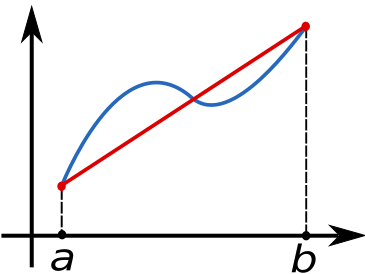
Trapezoidal rule. Join the points with straight lines:
\int_a^b f\,dx \approx \frac h2\big[f_0+2f_1+2f_2+\cdots+2f_{n-1}+f_n\big]
Error proportional to h^2.
Simpson's rule. Fit parabolas through groups of three points instead:
\int_a^b f\,dx\approx\frac h3\big[f_0+4f_1+2f_2+4f_3+\cdots+4f_{n-1}+f_n\big]
The alternating 4s and 2s look arbitrary and are what the parabola fitting produces.
Error proportional to h^4, which is an enormous improvement. Halving the step reduces the error by a factor of 16 rather than 4.
Worked comparison. \int_0^1 x^2 dx, whose exact value is \frac13, with 4 intervals:
Trapezoidal: \frac{0.25}{2}[0 + 2(0.0625)+2(0.25)+2(0.5625)+1] = 0.34375. Error 3%.
Simpson: \frac{0.25}{3}[0+4(0.0625)+2(0.25)+4(0.5625)+1] = 0.33333. Exact.
Simpson is exact for anything up to a cubic — it fits parabolas, and the cubic error term cancels by symmetry — which is why it is the default for smooth functions.
Gaussian quadrature does better still by choosing where to sample rather than using evenly spaced points. With n well-chosen points it integrates polynomials up to degree 2n-1 exactly. This is what library integrators use, and the sample points come from the orthogonal polynomials of Chapter 9.1.
Adaptive quadrature subdivides where the function is difficult and takes large steps where it is smooth, by comparing the estimate from one step against the estimate from two half-steps and refining when they disagree. Every quad function in every numerical library works this way.
Monte Carlo integration takes a completely different approach: sample randomly and average.
\int_V f\,dV \approx V\cdot\frac1N\sum f(\mathbf{x}_i)
Its error falls as \frac{1}{\sqrt N} — Chapter 7.4's square-root law — which is dreadful in one dimension and independent of the number of dimensions, which is spectacular in high ones. A grid method in 20 dimensions with just 10 points per axis needs 10^{20} evaluations. Monte Carlo needs however many it needs and does not care about the dimension count.
This is why Monte Carlo runs finance, particle physics and light transport in rendering. Every ray-traced image is a Monte Carlo integral over all the light paths reaching each pixel, and the characteristic grainy noise of an under-sampled render is the \frac{1}{\sqrt N} error, visible.
3. Solving differential equations numerically
Given \frac{dy}{dt} = f(t,y) with a starting value, step forward in time.
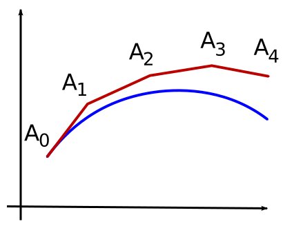
Euler's method. Use the slope at the current point and take a step:
y_{n+1} = y_n + h\,f(t_n,y_n)
Simple, first-order accurate, and generally too inaccurate for real use — but it is the honest picture of what every solver is doing.
Runge–Kutta 4 (RK4) is the workhorse. It evaluates the slope four times per step — at the start, twice in the middle, and at a trial endpoint — and takes a weighted average:
k_1 = f(t_n,y_n)
k_2 = f(t_n+\tfrac h2,\; y_n+\tfrac h2k_1)
k_3 = f(t_n+\tfrac h2,\; y_n+\tfrac h2k_2)
k_4 = f(t_n+h,\; y_n+hk_3)
y_{n+1} = y_n + \frac h6(k_1+2k_2+2k_3+k_4)
Fourth-order accurate. Halving the step cuts the error by 16. Four function evaluations buy an enormous accuracy gain over four Euler steps, and RK4 is the default in most engineering software.
Adaptive step size. Modern solvers estimate the local error by comparing two methods of different order and adjust h automatically — small steps through rapid changes, large steps through quiet stretches. This is what ode45 in MATLAB and solve_ivp in SciPy do.
4. Stiffness
Some systems have processes on wildly different time scales — a chemical reaction with one step in microseconds and another in hours, or a circuit with a fast transient and a slow settling.
These are stiff, and an ordinary explicit method is forced to take steps small enough for the fastest process even long after that process has finished. Simulating one hour at microsecond steps is a billion steps.
The fix is an implicit method. Backward Euler uses the slope at the end of the step:
y_{n+1} = y_n + h\,f(t_{n+1},y_{n+1})
The unknown appears on both sides, so each step requires solving an equation — Chapter 10.2's Newton's method, every step. That is far more expensive per step, and it is stable at step sizes that would make an explicit method explode, so the total cost is far lower.
Recognising stiffness matters because the symptom is confusing. A simulation that runs impossibly slowly, or that blows up to infinity for no visible reason, is usually stiff rather than wrong. Switching to a stiff solver is the fix, and it is the single most useful piece of practical knowledge in this chapter.
5. Partial differential equations
Finite differences. Put a grid over space and time, replace every derivative with a difference formula from Section 1, and step forward. Simple, and restricted to regular geometries.
Stability is a hard constraint. For the heat equation, an explicit scheme is stable only when
\frac{\alpha\,\Delta t}{(\Delta x)^2} \le \frac12
Halving the grid spacing forces the time step down by a factor of four. Refining a simulation therefore costs far more than it looks — twice the resolution in one dimension means eight times the work. This is the Courant–Friedrichs–Lewy condition, and it is why implicit methods are standard for diffusion problems.
Finite elements. Break the region into small triangles or tetrahedra, approximate the solution by simple functions on each, and assemble one enormous sparse linear system. This is what every structural, thermal, fluid and electromagnetic analysis package runs, and it handles complicated geometry, which finite differences cannot.
The assembled system is solved by the sparse and iterative methods of Chapter 4.3. A car crash simulation is millions of elements and hundreds of thousands of time steps, and it is Chapter 4.3 and this chapter, at scale.
Spectral methods expand in a Fourier basis (Chapter 9.2) and are extremely accurate for smooth problems on simple domains. Weather models use them for the global atmosphere.
6. What to actually trust
Convergence testing. Run at one resolution, then at half the step, and compare. If the answers agree to your required accuracy, the discretisation error is small. If they do not, refine further. Never report a number from a single resolution.
Conservation checks. If the physics conserves energy, mass or momentum, check that the simulation does. A drift in a conserved quantity is the clearest possible signal that something is wrong.
Symplectic integrators, for orbital and molecular mechanics, are designed to conserve energy over very long runs even at the cost of local accuracy. Ordinary RK4 will slowly gain or lose energy, so a simulated planet spirals into or away from its star over millions of steps — not because the physics says so but because the integrator leaks. This matters enormously for long simulations and not at all for short ones.
Sanity checks against known cases. Run the solver on a problem with a known answer before trusting it on one without.
Every formula above, built from scratch
None of the results in this chapter are worth memorising, because each one can be rebuilt in under a minute from something simpler. What follows is that rebuilding, one result at a time, so the formula and the reason for it sit on the same page as the explanation that needed them.
Numerical calculus
Derivatives by differences
f'(x)\approx\frac{f(x+h)-f(x)}{h} \qquad \text{error } O(h)
f'(x)\approx\frac{f(x+h)-f(x-h)}{2h} \qquad \text{error } O(h^2)
f''(x)\approx\frac{f(x+h)-2f(x)+f(x-h)}{h^2} \qquad \text{error } O(h^2)
Why the central difference is better. Expand both terms with Taylor:
f(x+h) = f+hf'+\tfrac{h^2}{2}f''+\tfrac{h^3}{6}f'''+\cdots
f(x-h) = f-hf'+\tfrac{h^2}{2}f''-\tfrac{h^3}{6}f'''+\cdots
Subtract. The f terms cancel, and so do the f'' terms, because they have the same sign in both:
f(x+h)-f(x-h) = 2hf'+\tfrac{h^3}{3}f'''+\cdots
Divide by 2h. The leading error term carries h^2, not h. The symmetric error terms cancelled, which is why symmetry is worth seeking in every numerical formula.
The trap that catches everyone: smaller h is not always better. Two errors compete.
\text{total error} \approx \underbrace{Ch^2}_{\text{truncation}} + \underbrace{\frac{\varepsilon|f|}{h}}_{\text{rounding}}
Truncation error falls as h shrinks; rounding error grows, because you are subtracting two nearly equal numbers and dividing by something tiny. Minimising the sum gives an optimal step of roughly h\approx\varepsilon^{1/3}\approx6\times10^{-6} for the central difference, at which point you get about 10 correct digits — and never more. Asking for h = 10^{-15} gives a worse answer than h = 10^{-5}.
Integration rules
\text{Trapezoid: } \int_a^b f \approx \frac h2\left[f_0+2f_1+\cdots+2f_{n-1}+f_n\right], \qquad \text{error } -\frac{(b-a)h^2}{12}f''(\xi)
\text{Simpson: } \int_a^b f\approx\frac h3\left[f_0+4f_1+2f_2+4f_3+\cdots+f_n\right], \qquad \text{error } -\frac{(b-a)h^4}{180}f^{(4)}(\xi)
Where the trapezoid rule comes from. Replace the curve on each strip with the straight line joining its endpoints. A trapezium of width h and heights f_i, f_{i+1} has area \frac h2(f_i+f_{i+1}). Adding them makes every interior height appear twice, which is where the 2's come from.
Where Simpson's rule comes from. Fit a parabola through three consecutive points instead of a line through two. Integrating that parabola over the two strips gives \frac h3(f_i+4f_{i+1}+f_{i+2}), and chaining them produces the 1,4,2,4,\ldots,4,1 pattern. It needs an even number of strips.
What the error terms tell you. Trapezoid error scales as h^2: halve the step and the error falls fourfold. Simpson scales as h^4: halve the step and the error falls sixteen-fold. And because Simpson's error involves the fourth derivative, it is exact for any cubic — a fact that surprises people, since it was built from parabolas.
\text{Richardson extrapolation: } I \approx \frac{4I_{h/2}-I_h}{3}
Combine two trapezoid estimates so the h^2 error terms cancel, and what remains is h^4 accurate. Doing this repeatedly is Romberg integration, and the first step of it is Simpson's rule.
\text{Gaussian quadrature: } \int_{-1}^{1}f(x)dx\approx\sum_{i=1}^n w_if(x_i)
Instead of evenly spaced points, choose both the positions and the weights optimally. With n points it integrates any polynomial of degree 2n-1 exactly — twice the degree you would expect. Two points, placed at \pm\frac{1}{\sqrt3} with weights 1, integrate any cubic perfectly.
Solving differential equations numerically
\text{Euler: } y_{n+1} = y_n + hf(t_n,y_n) \qquad \text{error } O(h)
Take the slope at the current point and walk along it. Simple, and rarely accurate enough.
\text{Runge–Kutta 4: } y_{n+1} = y_n+\frac h6\left(k_1+2k_2+2k_3+k_4\right)
k_1 = f(t_n,y_n), \quad k_2 = f\!\left(t_n+\tfrac h2, y_n+\tfrac h2k_1\right), \quad k_3 = f\!\left(t_n+\tfrac h2,y_n+\tfrac h2k_2\right), \quad k_4 = f(t_n+h,y_n+hk_3)
What it is doing. Sampling the slope four times across the step — once at the start, twice in the middle, once at the end — and taking a weighted average, with the middle samples counted double. The middles get more weight because they represent the interval better than either end. The error is O(h^4), which is why RK4 is the default in almost every simulation.
Stiff equations are the exception: when a system contains both very fast and very slow parts, explicit methods need a step small enough for the fast part even after it has died away, which makes them impossibly slow. Implicit methods, which solve for y_{n+1} on both sides, handle this and are what chemical kinetics and circuit simulators use.
7. Where this shows up in your life
Every weather forecast, crash test, and aerodynamic design.
Every game's physics engine, which is a fast, cheap, deliberately inaccurate differential equation solver — accurate enough to look right, fast enough to run 60 times a second.
Every rendered film frame. Monte Carlo light transport.
Every option priced and every risk figure computed in finance. Monte Carlo over price paths.
Every drug simulation and every molecular dynamics run.
Every spacecraft trajectory. Symplectic integrators, because the simulation must stay honest over years.
Solving equations is one problem. Finding the best solution among many is another, and it is the one that trains every model and designs every system.