Appearance
6.1 — What a Differential Equation Is
A cup of tea at 90°C sits in a 20°C room. How hot is it in ten minutes?
Nobody can write down the answer directly. What you can write down is the rule governing it, and Newton found it in the 1700s: the rate at which something cools is proportional to how much hotter it is than its surroundings. A very hot cup loses heat fast; a nearly-cool one loses heat slowly.
In symbols, with T the temperature and t the time:
\frac{dT}{dt} = -k(T - 20)
The minus sign says the temperature falls when the tea is hotter than the room, and k is a positive constant that depends on the cup and the tea.
This is a differential equation — an equation containing a derivative. Its unknown is not a number but a function. Solving it means finding the whole temperature curve, not one value.
And this is why calculus matters so much to science. The laws of nature are almost never statements about quantities. They are statements about rates: how fast something moves, decays, spreads, cools, charges or grows. Newton's second law, Maxwell's equations, the Schrödinger equation, the equations of fluid flow, and every model in epidemiology and finance are differential equations. Writing the rule is often easy; extracting the behaviour is the work.
1. Vocabulary, quickly
Order is the highest derivative present. The tea equation is first order. Anything involving acceleration is second order, which is Chapter 6.2.
Ordinary (an ODE) means one independent variable, so only ordinary derivatives appear. Partial (a PDE) means several, so partial derivatives appear. Chapter 6.4 covers those.
Linear means the unknown function and its derivatives appear only to the first power and are never multiplied together. Linear equations are vastly easier, because solutions can be added: if y_1 and y_2 both solve the equation, so does y_1 + y_2. That property, called superposition, is the foundation of almost every solution technique in this Part and of the transforms in Part 9.
Nonlinear loses superposition and with it almost all general methods. Most real systems are nonlinear, which is why so much of applied mathematics is the art of finding a linear approximation that is good enough.
General versus particular. A differential equation has a family of solutions with an arbitrary constant in it — this is Chapter 5.5's +C, and it means the same thing: the rate alone does not fix the starting point. An initial condition picks one member of the family.
2. Separable equations
The simplest solvable type: everything with y can be moved to one side and everything with t to the other.
\frac{dy}{dt} = f(t)g(y) \quad\Longrightarrow\quad \int\frac{dy}{g(y)} = \int f(t)\,dt
Worked example: the tea.
\frac{dT}{dt} = -k(T-20)
Separate:
\frac{dT}{T-20} = -k\,dt
Integrate both sides, using Chapter 5.5's \int\frac{1}{x}dx = \ln|x|:
\ln|T-20| = -kt + C
Undo the logarithm by exponentiating:
T - 20 = Ae^{-kt}, \qquad\text{where } A = e^C
T(t) = 20 + Ae^{-kt}
Apply the initial condition. At t=0 the tea is at 90°C, so 90 = 20 + A, giving A = 70:
T(t) = 20 + 70e^{-kt}
Interpret it before computing anything. The tea starts 70 degrees above the room and that excess decays exponentially. It approaches 20°C and never quite reaches it — mathematically, at least; physically it becomes indistinguishable long before.
Suppose measurement shows the tea at 60°C after 5 minutes. Then 40 = 70e^{-5k}, so e^{-5k} = 0.571, so k = \frac{\ln(70/40)}{5} = 0.112 per minute. At t = 10:
T = 20 + 70e^{-1.12} = 20 + 22.9 = 42.9°\text{C}
Why adding cold milk early keeps your tea hotter
Suppose you must leave the tea for ten minutes before drinking, and you want it as hot as possible. Add the milk now, or at the end?
Add it now. Milk immediately drops the temperature, which reduces the gap to the room, which by Newton's law slows the subsequent cooling. Over the ten minutes the tea-with-milk loses less heat than the black tea would, and the final temperature is higher than if you had cooled a hotter cup at the end.
This is a genuine and testable consequence of the equation, and it is the everyday version of the point that the rate depends on the current state, which is what makes these equations interesting.
3. The one equation that describes everything
\frac{dy}{dt} = ky \quad\Longrightarrow\quad y = y_0e^{kt}
The rate of change is proportional to the current amount. This is the most important differential equation in the sciences, and its solution is why the exponential function is everywhere.
| k | Behaviour | Where |
|---|---|---|
| k \gt 0 | growth | population, compound interest, viral spread |
| k \lt 0 | decay | radioactivity, drug clearance, cooling, capacitor discharge |
Radioactive decay. Each nucleus has a fixed chance of decaying per unit time, independent of age, so the number decaying is proportional to the number present: \frac{dN}{dt} = -\lambda N.
The half-life is when half remains: \frac12 = e^{-\lambda t_{1/2}}, so
t_{1/2} = \frac{\ln 2}{\lambda}
The same \ln 2 as the rule of 72 in Chapter 1.4, doing the same job.
Carbon dating uses this. Living things maintain a fixed proportion of carbon-14; when they die, it decays with a half-life of 5,730 years. A sample with 25% of the expected carbon-14 has been through two half-lives, so it is about 11,460 years old. Same equation, read backwards.
Compound interest. Chapter 1.3's discrete formula becomes \frac{dA}{dt} = rA when compounding is continuous, with solution A = Pe^{rt} — and Chapter 1.4's definition of e was exactly this limit.
Drug half-life. Why a medicine is taken every eight hours: the dose decays exponentially, and the interval is chosen so the concentration stays inside the therapeutic window between doses.
4. Logistic growth: what happens when resources run out
Exponential growth cannot continue. Bacteria run out of food; a market saturates; a virus runs out of susceptible people. The fix is one extra factor:
\frac{dP}{dt} = rP\left(1 - \frac{P}{K}\right)
K is the carrying capacity. When P is small compared to K, the bracket is nearly 1 and growth is exponential. As P approaches K, the bracket approaches zero and growth stops.
The solution is the logistic curve, an S-shape: slow start, rapid middle, levelling off. The steepest point is at exactly half the carrying capacity.
This one curve describes bacterial cultures, the adoption of new technology, tumour growth, the spread of an epidemic through a fixed population, and product sales over a lifecycle. It is also the activation function that gave early neural networks their name — the sigmoid of Volume I, 12.4 is this curve.
And it is nonlinear, because of the P^2 hidden in the bracket. Solving it still works by separation, needing the partial fractions of Chapter 5.6, and this is one of the few nonlinear equations with a clean closed-form solution.
5. Linear first-order equations
\frac{dy}{dt} + p(t)y = q(t)
Not separable in general. The method: multiply through by an integrating factor \mu = e^{\int p\,dt}, chosen precisely so the left side becomes the derivative of a product:
\frac{d}{dt}(\mu y) = \mu q
Then integrate both sides.
Worked example. \frac{dy}{dt} + 2y = 6, with y(0) = 1.
Here p = 2, so \mu = e^{2t}:
\frac{d}{dt}(e^{2t}y) = 6e^{2t} \quad\Longrightarrow\quad e^{2t}y = 3e^{2t} + C \quad\Longrightarrow\quad y = 3 + Ce^{-2t}
With y(0) = 1: C = -2, so y = 3 - 2e^{-2t}.
Read the shape. The solution has two parts: a steady state of 3, which is where it settles, and a transient -2e^{-2t}, which dies away. Every stable linear system behaves this way — a transient that fades and a steady state that persists. It is why a light does not reach full brightness instantly, why a thermostat overshoots and settles, and why a circuit takes time to charge.
That decomposition into transient plus steady state is the central idea of control engineering, and Chapter 9.5's Laplace transform is the tool that separates them mechanically.
6. Direction fields: seeing the solution without solving
Even when you cannot solve an equation, you can see what its solutions look like.
At each point of the plane, \frac{dy}{dt} = f(t,y) gives a slope. Draw a short line segment with that slope at many points, and you have a direction field. Any solution curve must flow along those segments.
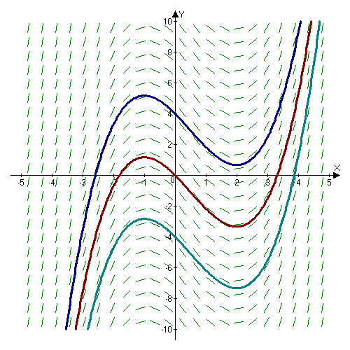
Equilibrium solutions are where the derivative is zero — constant solutions. For the logistic equation these are P=0 and P=K.
They come in two kinds, and the distinction matters more than the values.
Stable: nearby solutions move towards it. Push the system slightly and it returns. P = K is stable.
Unstable: nearby solutions move away. Push it slightly and it runs off. P = 0 is unstable — introduce a single bacterium and the population takes off.
A pencil balanced on its point is an unstable equilibrium; hanging from a string it is stable. Deciding which is which is often the whole question in engineering, ecology and economics, and Chapter 6.3 does it systematically.
Every formula above, built from scratch
None of the results in this chapter are worth memorising, because each one can be rebuilt in under a minute from something simpler. What follows is that rebuilding, one result at a time, so the formula and the reason for it sit on the same page as the explanation that needed them.
The vocabulary, in one place
\text{order} = \text{the highest derivative present}
\text{linear}: \quad a_n(x)y^{(n)} + \cdots + a_1(x)y' + a_0(x)y = f(x)
Linear means y and its derivatives appear only to the first power, never multiplied together, never inside a sine or a square root. y'' + 3y = \cos x is linear; y'' + y^2 = 0 and yy' = 1 are not. Linearity is the property that makes solutions add, and almost every technique below depends on it.
A general solution to an n-th order equation contains n arbitrary constants. Fixing them needs n extra facts, called initial conditions when they are all given at the same point and boundary conditions when they are given at different points.
Separable equations
\frac{dy}{dx} = g(x)h(y) \quad \Longrightarrow \quad \int\frac{dy}{h(y)} = \int g(x)\,dx
Where the method comes from. Divide both sides by h(y) and multiply by dx:
\frac{dy}{h(y)} = g(x)\,dx
Now integrate both sides. The left is an integral in y alone, the right in x alone, and each can be done separately. Treating \frac{dy}{dx} as a fraction looks like cheating; the honest version integrates \frac{1}{h(y)}\frac{dy}{dx} with respect to x and uses the substitution rule, which produces the same two integrals. The shortcut is legitimate, and Leibniz designed the notation so that it would be.
The worked archetype. \frac{dy}{dx} = ky:
\int\frac{dy}{y} = \int k\,dx \quad \Rightarrow \quad \ln|y| = kx + C
Exponentiate both sides:
|y| = e^{kx+C} = e^Ce^{kx}
Since e^C is just some positive constant, and the absolute value allows either sign, write it as a single constant A:
y = Ae^{kx}
Putting x=0 shows A = y(0), the starting value. This is the most important solution in applied mathematics, and everything in §3 is a variation on it.
First-order linear equations
\frac{dy}{dx}+P(x)y = Q(x)
\text{Integrating factor: } \mu(x) = e^{\int P(x)dx}, \qquad y = \frac{1}{\mu}\int \mu Q\,dx
Where the integrating factor comes from — and it is a genuinely clever idea, not a rule. The problem is that the left-hand side is almost the derivative of a product but not quite. So multiply the whole equation by some unknown function \mu(x) and see what \mu would have to be to fix that:
\mu y' + \mu Py = \mu Q
We want the left side to be exactly \frac{d}{dx}(\mu y). By the product rule,
\frac{d}{dx}(\mu y) = \mu y' + \mu' y
Comparing the two lines, they agree if and only if
\mu' = \mu P
That is a separable equation for \mu, and §2 solves it immediately:
\frac{d\mu}{\mu} = P\,dx \quad \Rightarrow \quad \ln\mu = \int P\,dx \quad \Rightarrow \quad \mu = e^{\int P dx}
With that \mu, the equation has become
\frac{d}{dx}(\mu y) = \mu Q
and both sides can simply be integrated:
\mu y = \int\mu Q\,dx \quad \Rightarrow \quad y = \frac{1}{\mu}\int\mu Q\,dx
Nothing was assumed. The factor was derived by demanding that the product rule apply.
Two more first-order forms
Homogeneous (every term the same total degree): if \frac{dy}{dx} = F\left(\frac yx\right), substitute v = \frac yx, so y = vx and y' = v + xv'. The equation becomes separable in v.
Bernoulli: y' + P y = Qy^n. Divide by y^n and substitute u = y^{1-n}. Then u' = (1-n)y^{-n}y', and the equation becomes linear in u:
u' + (1-n)Pu = (1-n)Q
Exact equations: M\,dx + N\,dy = 0 is exact when \frac{\partial M}{\partial y} = \frac{\partial N}{\partial x}, and the solution is F(x,y) = C where F_x = M and F_y = N. The test works because mixed partial derivatives of a smooth function are equal, so that condition is exactly what allows such an F to exist.
The standard models, each solved
Exponential growth and decay
\frac{dN}{dt} = kN \quad \Rightarrow \quad N(t) = N_0e^{kt}
\text{Half-life: } t_{1/2} = \frac{\ln 2}{|k|}
Where the half-life formula comes from. Set N = \frac{N_0}{2}:
\frac{N_0}{2} = N_0e^{kt} \quad \Rightarrow \quad \frac12 = e^{kt} \quad \Rightarrow \quad \ln\frac12 = kt \quad \Rightarrow \quad t = \frac{-\ln2}{k}
For decay k is negative, so the time comes out positive.
Newton's law of cooling
\frac{dT}{dt} = -k(T - T_s) \quad \Rightarrow \quad T(t) = T_s + \left(T_0-T_s\right)e^{-kt}
Where the solution comes from. The equation says the cooling rate is proportional to how much hotter the object is than its surroundings. Substitute u = T - T_s, the excess temperature. Since T_s is constant, \frac{du}{dt} = \frac{dT}{dt}, and the equation becomes
\frac{du}{dt} = -ku
which is the archetype of §2, giving u = u_0e^{-kt}. Translate back:
T - T_s = (T_0-T_s)e^{-kt}
Read the answer. The object's temperature is the room's temperature, plus the initial gap, shrinking exponentially. It never quite reaches room temperature in the model, but the gap halves every \frac{\ln2}{k}, so in practice it does. This is the equation forensic scientists use to estimate a time of death, and it is why a cup of coffee cools fastest in its first minute.
The logistic equation
\frac{dP}{dt} = rP\left(1-\frac PK\right) \quad \Rightarrow \quad P(t) = \frac{K}{1 + \left(\frac{K-P_0}{P_0}\right)e^{-rt}}
What the equation says. Growth is proportional to the population, as before, but multiplied by a brake \left(1-\frac PK\right) that closes as P approaches the carrying capacity K. When P is tiny the brake is nearly 1 and growth is nearly exponential; when P reaches K the brake is zero and growth stops.
Where the solution comes from — worth following, because the partial fractions step is the whole trick. Separate:
\frac{dP}{P\left(1-\frac PK\right)} = r\,dt \quad \Rightarrow \quad \frac{K\,dP}{P(K-P)} = r\,dt
Split the left with partial fractions. Since \frac{K}{P(K-P)} = \frac{A}{P}+\frac{B}{K-P}, clearing denominators gives K = A(K-P)+BP. Put P=0: K = AK, so A = 1. Put P=K: K = BK, so B=1.
\int\left(\frac1P + \frac{1}{K-P}\right)dP = \int r\,dt
\ln|P| - \ln|K-P| = rt + C
The minus on the second term comes from the chain rule: the derivative of K-P with respect to P is -1.
\ln\left|\frac{P}{K-P}\right| = rt+C \quad \Rightarrow \quad \frac{P}{K-P} = Ae^{rt}
Solve for P:
P = Ae^{rt}(K-P) \quad \Rightarrow \quad P\left(1+Ae^{rt}\right) = AKe^{rt} \quad \Rightarrow \quad P = \frac{AKe^{rt}}{1+Ae^{rt}}
Divide top and bottom by Ae^{rt} to get the standard form, and use t=0 to identify A = \frac{P_0}{K-P_0}:
P(t) = \frac{K}{1+\left(\frac{K-P_0}{P_0}\right)e^{-rt}}
The S-shape, and where its bend is. The curve rises slowly, then steeply, then levels off. The steepest point — the inflection — is at exactly P = \frac K2, which you can see by differentiating the growth rate rP(1-P/K) with respect to P and setting it to zero. Half capacity is where a population, an epidemic, or the adoption of a new technology is growing fastest, and it is the moment forecasters most often mistake for the beginning of unbounded growth.
Mixing problems
\frac{dA}{dt} = (\text{rate in}) - (\text{rate out}) = c_{\text{in}}r_{\text{in}} - \frac{A}{V(t)}r_{\text{out}}
The concentration flowing out is whatever is currently in the tank, \frac AV, which is what makes this a differential equation rather than arithmetic. If the volume is constant this is first-order linear and §3 solves it.
7. Where this shows up in your life
Every cooling and heating calculation. Your tea, your fridge, your engine, the cooling of a data centre.
Every drug schedule. Half-life determines dosing intervals, and loading doses exist because the steady state takes several half-lives to reach.
Every carbon date and every radiometric age. The Earth's age of 4.54 billion years comes from exactly this equation applied to uranium-lead decay.
Every epidemic model. The exponential early phase, then logistic saturation, and R_0 as the growth constant.
Every capacitor charging in every device you own. V = V_0(1-e^{-t/RC}), which is Section 5's transient-plus-steady-state solution. Volume III, 1.5.
Every interest and depreciation calculation done continuously.
First-order equations describe things that settle. Nothing here can oscillate — no solution wobbles, rings or resonates. For that you need a second derivative, and with it comes the phenomenon that has knocked down bridges.