Appearance
10.4 — Optimization: Finding the Best Answer
Every trained machine learning model, every engineering design, every portfolio allocation and every delivery route is the answer to the same question: among all the possibilities, which one is best?
Chapter 5.4 answered it for one variable with calculus — set the derivative to zero and solve. That works when you can solve the equation and there are a handful of variables. A modern language model has hundreds of billions of parameters and a loss function nobody can write down in closed form.
So you do not solve. You walk downhill.
1. The problem, stated
Minimise f(\mathbf{x}) over \mathbf{x}, possibly subject to constraints.
Maximising is minimising the negative, so one formulation covers both. f is called the objective function, or in machine learning the loss.
The distinction that governs everything: convex or not.
A function is convex if the straight line between any two points on its graph lies above the graph — a bowl shape, with no dents.
For a convex function, any local minimum is the global minimum. Walk downhill from anywhere and you arrive at the answer. There is nowhere else to get stuck.
For a non-convex function there is no such guarantee. You may land in a local minimum that is far worse than the best one, and finding the global minimum of a general non-convex function is intractable.
This is the single most important question to ask about an optimisation problem, because it determines whether you have a reliable method or a heuristic.
2. Gradient descent
Chapter 5.7 gave the gradient: the vector of partial derivatives, pointing in the direction of steepest increase. So the opposite direction is steepest decrease.
\mathbf{x}_{n+1} = \mathbf{x}_n - \eta\,\nabla f(\mathbf{x}_n)
Take a small step downhill. Repeat. That is the whole algorithm, and it trains essentially every model in modern machine learning.
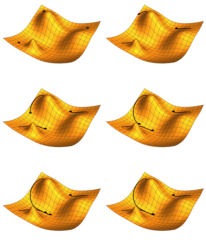
The learning rate \eta is the whole difficulty.
Too large and the steps overshoot the valley floor, bouncing between the walls or diverging to infinity. Too small and it takes forever and may stall on a flat stretch.
The zigzag problem. In a long narrow valley, the gradient points mostly across the valley rather than along it, so the path oscillates between the walls and creeps slowly towards the minimum. The severity is governed by the condition number of the Hessian — Chapter 10.1's quantity again, in a new setting.
The refinements that make it work
Momentum. Accumulate a velocity rather than stepping fresh each time:
\mathbf{v}_{n+1} = \beta\mathbf{v}_n - \eta\nabla f, \qquad \mathbf{x}_{n+1} = \mathbf{x}_n+\mathbf{v}_{n+1}
Like a ball rolling downhill. Consistent directions accumulate speed; oscillating directions cancel out. This kills the zigzag and accelerates progress along the valley floor.
Adaptive learning rates. AdaGrad, RMSProp and Adam give each parameter its own step size, based on the size of the gradients it has been receiving. Parameters with large gradients get small steps and parameters with small gradients get large ones, which handles the case where different parameters need wildly different scales.
Adam combines momentum with adaptive rates and is the default optimiser for most deep learning. Volume I, 12.4 covers the practice.
Stochastic gradient descent. With a million training examples, computing the exact gradient means evaluating all million every step. Instead, use a random mini-batch of perhaps 32 or 256.
The gradient estimate is noisy, and it is a hundred thousand times cheaper. You take vastly more steps in the same time, and the noise turns out to help — it can jolt the iterate out of a poor local minimum or off a saddle point. Volume I, 12.4.
3. Using second derivatives
Gradient descent uses only the slope. The curvature tells you how far to step.
Newton's method for optimisation is Chapter 10.2's root-finder applied to \nabla f = 0:
\mathbf{x}_{n+1} = \mathbf{x}_n - H^{-1}\nabla f
where H is the Hessian of second derivatives (Chapter 5.7).
Quadratic convergence, so it is dramatically faster near the answer. And it is unusable at scale: the Hessian for n parameters has n^2 entries, so a billion-parameter model would need 10^{18} numbers.
Quasi-Newton methods build an approximation to the inverse Hessian from the gradients already computed. BFGS is the standard, and L-BFGS ("limited memory") stores only the last few updates instead of a full matrix. L-BFGS is the default for medium-sized problems — thousands to millions of parameters — and it is what scipy.optimize.minimize uses unless told otherwise.
Which to use, honestly:
| Problem size | Method |
|---|---|
| Small, smooth, convex | Newton or BFGS |
| Medium, smooth | L-BFGS |
| Huge, noisy, non-convex | SGD with momentum, or Adam |
| No derivatives available | Nelder–Mead, or a metaheuristic |
4. Constrained optimisation
Real problems have limits. Budgets, capacities, physical bounds, requirements.
Equality constraints use the Lagrange multipliers of Chapter 5.7: at the optimum, the objective's gradient is parallel to the constraint's gradient.
Inequality constraints generalise this to the Karush–Kuhn–Tucker conditions, whose key idea is simple: a constraint either binds at the optimum or it does not. If it binds, it behaves like an equality constraint and gets a multiplier. If it does not, it might as well not exist and its multiplier is zero.
The multiplier is the shadow price — how much the objective would improve if you relaxed that constraint by one unit. This is what an operations manager actually wants to know: which constraint is costing the most, and therefore which is worth spending money to relax.
Penalty methods convert a constrained problem into an unconstrained one by adding a large cost for violation. Crude and effective, and it is what regularisation in machine learning is: adding a penalty on the size of the weights is a soft constraint keeping them small, which prevents overfitting.
5. When there are no derivatives
Sometimes the function is a simulation, a physical experiment, or a black box.
Nelder–Mead maintains a simplex — a triangle in two dimensions, a tetrahedron in three — and repeatedly reflects the worst vertex through the others, expanding when things improve and contracting when they do not. Slow, derivative-free, and remarkably robust. It is a reasonable first choice for a small messy problem.
Simulated annealing takes random steps and accepts uphill moves with a probability that decreases over time, controlled by a "temperature" parameter. Early on it wanders freely and escapes local minima; later it settles. The name and the schedule come from metallurgy, where cooling metal slowly lets the atoms find a low-energy crystal structure rather than freezing into defects.
Genetic algorithms maintain a population of candidate solutions, keep the better ones, combine them and randomly mutate. Inspired by evolution.

Metaheuristics, assessed honestly
Nature-inspired optimisers are enormously popular in the literature. Particle swarm, ant colony, artificial bee colony, grey wolf, whale, firefly, bat, cuckoo search — hundreds have been published, most differing from each other only in the metaphor.
Here is the honest assessment.
They have real uses. When the objective is a black box with no derivatives, when the space is discrete or combinatorial, or when you need a good answer quickly and cannot prove optimality, they are reasonable and sometimes the only option. Ant colony optimisation is genuinely good on some routing problems.
They come with no guarantees. No convergence proof, no bound on how far from optimal you are, and heavy sensitivity to parameters you must tune by hand.
They are usually beaten by a proper method when one applies. If your problem is convex, use a convex solver. If it is a linear program, use the simplex method. If gradients exist, use them. Reaching for a swarm when the derivative is available is a mistake, and the fact that the metaphor is charming is not an argument.
The literature has a real quality problem. A widely cited 2015 critique argued that many of these algorithms are the same method dressed in new biological language, with the novelty in the metaphor rather than the mathematics. Treat a new nature-inspired optimiser with the scepticism you would apply to any claim that is easy to publish and hard to falsify.
6. Practical advice
Scale your variables. If one parameter ranges over 10^{-6} and another over 10^6, the problem is artificially ill-conditioned and every method will struggle. Rescaling is often the entire fix.
Try several starting points on a non-convex problem, and compare the results. If they all reach the same value, that is evidence. If they scatter, you have learned something important.
Plot the objective against iteration count. A curve that plateaus early means the learning rate is too small or you have converged; one that oscillates or diverges means it is too large. This single plot diagnoses most optimisation failures.
Check the gradient. Compare your analytic gradient against a numerical one from Chapter 10.3. A wrong gradient produces an optimiser that converges to nonsense, confidently, and it is one of the most common bugs in scientific code.
Ask whether the problem is convex before choosing a method. Linear and quadratic objectives with linear constraints are convex, and convex solvers on convex problems give guaranteed global optima quickly. It is worth reformulating a problem to make it convex if you can.
Every formula above, built from scratch
None of the results in this chapter are worth memorising, because each one can be rebuilt in under a minute from something simpler. What follows is that rebuilding, one result at a time, so the formula and the reason for it sit on the same page as the explanation that needed them.
Optimisation
\text{Gradient descent: } \mathbf{x}_{n+1} = \mathbf{x}_n - \alpha\nabla f(\mathbf{x}_n)
Why it works. The gradient points uphill fastest, as shown in 5.7 — multivariable calculus §10, so its negative points downhill fastest. The learning rate \alpha sets the step size, and its choice is the whole difficulty: too small and it crawls, too large and it overshoots and diverges.
\text{Convergence requires } \alpha < \frac{2}{L}, \text{ where } L \text{ is the largest curvature}
\text{Momentum: } \mathbf{v}_{n+1} = \beta\mathbf{v}_n - \alpha\nabla f, \qquad \mathbf{x}_{n+1} = \mathbf{x}_n+\mathbf{v}_{n+1}
Keeping a running average of past steps damps the zig-zagging that happens in a narrow valley, where the gradient points mostly across the valley rather than along it.
\text{Newton's method for optimisation: } \mathbf{x}_{n+1} = \mathbf{x}_n - H^{-1}\nabla f
Uses the Hessian of second derivatives to choose both the direction and the step length. Quadratically convergent, but the Hessian costs O(n^2) to store and O(n^3) to invert, so for a model with a million parameters it is out of the question. That is why machine learning uses gradient descent and its variants rather than the mathematically better method.
Convexity is what makes optimisation safe.
f \text{ convex} \iff f''\ge0 \iff \text{the Hessian is positive semi-definite}
For a convex function, any local minimum is the global minimum, so a downhill algorithm cannot be trapped. For a non-convex function there is no such guarantee, and the practical answer is to run from several starting points and keep the best.
\text{Constrained: } \nabla f = \sum\lambda_i\nabla g_i \quad\text{(Lagrange, from 5.F)}
with the KKT conditions extending this to inequality constraints: at the optimum, either a constraint is tight and has a non-negative multiplier, or it is slack and its multiplier is zero.
7. Where this shows up in your life
Every trained AI model. SGD or Adam, over billions of parameters.
Every route your delivery arrives by. Combinatorial optimisation with heuristics.
Every portfolio allocation. Markowitz's mean-variance optimisation is a quadratic program, and it won a Nobel Prize.
Every engineering design that minimises weight, cost or drag subject to strength and safety constraints.
Every airline schedule, hospital roster and power-plant dispatch.
Every curve fitted to data, from a spreadsheet trendline to a scientific model — least squares is optimisation, and Chapter 4.3 gave its closed form.
One family of optimisation problems is important enough, and well-behaved enough, to deserve separate treatment. It is also the one that generates the most economic value of any mathematics invented in the twentieth century.