Appearance
6.2 — Oscillation, Damping and Resonance
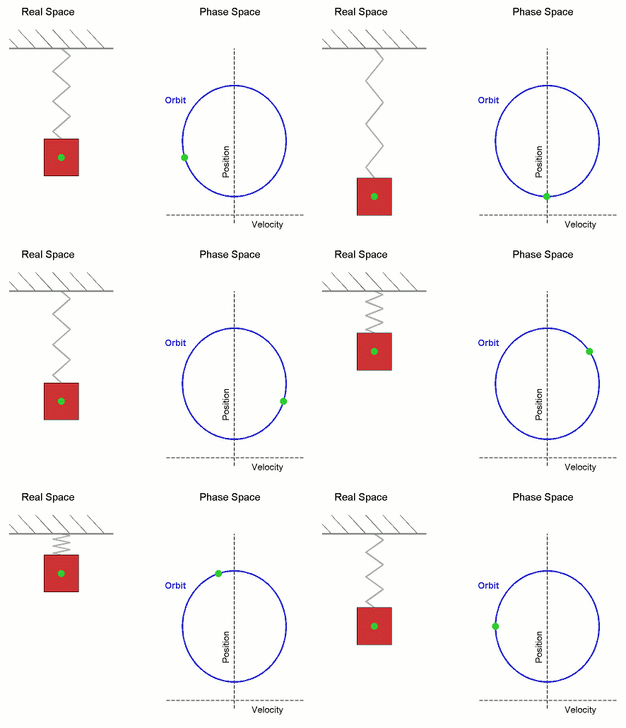
Pull a mass on a spring and let go. It does not settle quietly the way the tea in Chapter 6.1 did — it overshoots, comes back, overshoots again, and rings for a while before stopping.
Nothing in Chapter 6.1 can produce that. A first-order equation says the rate depends on the current state, and such a system always moves monotonically towards its equilibrium. To oscillate, a system needs to overshoot, and overshooting requires momentum, which requires a second derivative.
1. The equation of the spring
Hooke's law: a spring pulls back in proportion to how far it is stretched, F = -kx. Newton's second law: F = ma = m\ddot{x}, where the dots are Newton's notation for derivatives with respect to time (Chapter 5.2). Put them together:
m\ddot{x} = -kx \quad\Longrightarrow\quad \ddot{x} + \frac{k}{m}x = 0
Write \omega^2 = \frac{k}{m}:
\ddot{x} + \omega^2 x = 0
In words: the acceleration is proportional to the displacement, and opposite to it. The further you are from the middle, the harder you are pulled back.
What function has a second derivative equal to minus itself, up to a constant? Chapter 5.3 gives it: differentiate \sin twice and you get -\sin. So:
x(t) = A\cos(\omega t) + B\sin(\omega t) = C\sin(\omega t + \phi)
A sine wave. This is the answer Chapter 3.5 promised — sine waves are everywhere in nature not because nature has a taste for them, but because any restoring force proportional to displacement produces this equation, and this equation produces a sine.
\omega is the natural frequency, and \omega = \sqrt{k/m} says a stiffer spring oscillates faster and a heavier mass oscillates slower. Both match intuition.
The period is T = \frac{2\pi}{\omega} = 2\pi\sqrt{\frac{m}{k}}, and notice what is missing: the amplitude. How far you pull it does not change how long a swing takes. Galileo noticed this watching a lamp swing in Pisa cathedral, timing it against his own pulse, and it is the reason a pendulum can keep time at all.
The pendulum obeys \ddot\theta = -\frac{g}{L}\sin\theta, which is nonlinear because of the \sin. For small angles, Chapter 5.8's approximation \sin\theta\approx\theta turns it into the same equation with \omega = \sqrt{g/L}. So the period is 2\pi\sqrt{L/g} — depending on length and gravity, and not on mass or amplitude. For a 1 m pendulum that is 2.006 seconds, which is why grandfather clocks are the height they are.
The independence from amplitude fails for large swings, because the approximation fails. A pendulum clock therefore keeps good time only while its swing stays small, which is a real engineering constraint and not a footnote.
2. Damping: what friction does
Real oscillations die out. Add a resistance proportional to velocity — air drag, friction, electrical resistance:
m\ddot x + c\dot x + kx = 0
To solve, guess x = e^{rt}, which is the standard move for any linear equation with constant coefficients. Differentiating just multiplies by r, so substituting gives
mr^2 + cr + k = 0
A quadratic — the characteristic equation — and Chapter 2.3's discriminant now decides the entire physical behaviour.
| Discriminant c^2 - 4mk | Name | Behaviour |
|---|---|---|
| Negative | underdamped | oscillates, shrinking |
| Zero | critically damped | returns fastest, no overshoot |
| Positive | overdamped | returns slowly, no overshoot |
Underdamped (c^2 \lt 4mk): complex roots, which by Euler's formula (Chapter 2.5) means an oscillation multiplied by a decaying exponential:
x = Ae^{-\frac{c}{2m}t}\cos(\omega_d t + \phi)
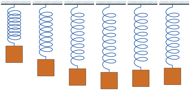
A ringing that fades. A plucked guitar string, a struck bell, a car with worn shock absorbers.
Critically damped: the fastest possible return to rest with no overshoot at all.
Overdamped: returns without overshooting, but sluggishly — like a door closer set too tight.
Critical damping is an engineering target, not an accident
Car suspension aims for slightly underdamped, close to critical. Too little damping and the car floats and wallows after every bump; too much and it transmits every jolt to the passengers. Worn shock absorbers reduce c, which is why an old car keeps bouncing after a speed bump — and why the standard test is to push down on a corner and count the bounces.
A door closer is deliberately overdamped so the door never slams.
A galvanometer needle or an analogue meter is critically damped so it reaches its reading in the shortest time without oscillating around it.
A digital control loop is tuned to the same target: settle fast, do not overshoot. The PID controller of Volume III, 6.6 exists to place a system at the right point on this scale.
Those damping regimes are much clearer moving than described. The slider below is the damping ratio, and everything else is held fixed.
Set the ratio to 1 and then to 1.5, and compare how long each takes to settle. The overdamped one is slower, which is the point that makes critical damping the target in almost every piece of engineering.
3. Forcing and resonance
Now push the system periodically:
m\ddot x + c\dot x + kx = F_0\cos(\omega_f t)
The solution is a transient that dies away plus a steady oscillation at the driving frequency, not the natural one. The system eventually does what it is told.
But the size of the response depends dramatically on how close the driving frequency is to the natural frequency. The amplitude is
A = \frac{F_0/m}{\sqrt{(\omega_0^2-\omega_f^2)^2 + \left(\frac{c\omega_f}{m}\right)^2}}
When \omega_f \approx \omega_0, the first bracket goes to zero and the amplitude is limited only by the damping. With small damping the response is enormous.
That is resonance: small repeated pushes at the right frequency build up a huge response, because each push arrives in step with the motion already there. Pushing a child on a swing is the everyday case — a small shove at exactly the right moment, every cycle, produces a large swing. Push at the wrong rhythm and you fight the motion.
Where resonance is used deliberately:
- A radio tuner. An LC circuit's resonant frequency is set by a variable capacitor; the station at that frequency produces a large response and everything else is ignored. That is what tuning is. Volume III, 1.6.
- An MRI scanner. Nuclear magnetic resonance excites hydrogen nuclei at their precise resonant frequency. The R in MRI is this word.
- A microwave oven drives water molecules near a rotational resonance, so energy goes into the food and mostly not into the plate.
- A musical instrument. The body of a guitar or violin resonates at frequencies that amplify the string's sound.
Where resonance destroys things:
- The Tacoma Narrows Bridge, 1940. Filmed twisting itself apart in a 65 km/h wind. The usual textbook explanation of simple resonance is an oversimplification — the accepted mechanism is aeroelastic flutter, where the bridge's own motion changed the airflow in a way that fed more energy in, a self-reinforcing loop rather than an external drive at a fixed frequency. The lesson is the same: a structure with too little damping near a driving frequency is in danger.
- The Millennium Bridge, London, 2000. It swayed sideways on opening day. Pedestrians instinctively adjusted their steps to match the sway, which reinforced it — again a feedback loop, this time through the people. It closed for two years and had dampers fitted.
- Marching soldiers break step on bridges, a standing order in most armies since the Broughton Suspension Bridge collapsed under marching troops in 1831.
- A wine glass shattered by a voice at its resonant frequency, which is real and requires both the right pitch and considerable volume.
The engineering discipline that follows: find every natural frequency of a structure and make sure no expected driving frequency lands near one. Those natural frequencies are the eigenvalues of Chapter 4.5, and computing them is a standard step in designing any bridge, building, aircraft or engine mount.
4. Electrical circuits are the same equation
An inductor, resistor and capacitor in series obey
L\ddot q + R\dot q + \frac{1}{C}q = V(t)
where q is charge. Compare with the mechanical equation term by term:
| Mechanical | Electrical |
|---|---|
| mass m | inductance L |
| damping c | resistance R |
| stiffness k | 1/C |
| force F | voltage V |
| displacement x | charge q |
Identical mathematics. Inductance resists changes in current the way mass resists changes in velocity; resistance dissipates energy the way friction does; a capacitor stores energy the way a spring does.
This is not a loose analogy — it is the same differential equation, so every result transfers. Engineers exploited it directly: before digital computers, mechanical systems were simulated by building the electrical circuit with the matching constants and measuring it. That machine was called an analogue computer, and it is where the word "analogue" comes from.
And it is why one branch of mathematics pays for itself across every field. Learning to solve a\ddot x + b\dot x + cx = f once means you have solved springs, circuits, pendulums, buildings in earthquakes, molecular vibrations and feedback control loops.
5. Solving these systematically
For a\ddot y + b\dot y + cy = f(t):
Step 1: the homogeneous solution. Set f = 0, solve the characteristic quadratic ar^2+br+c=0, and write down the solution according to the discriminant:
- Two real roots: y = Ae^{r_1t} + Be^{r_2t}.
- Repeated root: y = (A + Bt)e^{rt} — the extra t is needed to get two independent solutions.
- Complex roots \alpha\pm\beta i: y = e^{\alpha t}(A\cos\beta t + B\sin\beta t).
Step 2: a particular solution for the forcing f. Guess something of the same shape — a polynomial for a polynomial forcing, Ce^{kt} for an exponential, C\cos + D\sin for a sinusoid — and substitute to find the constants.
Step 3: add them. The general solution is homogeneous plus particular. This works because the equation is linear, so superposition holds.
Step 4: apply two initial conditions — usually position and velocity at t=0 — to fix the two constants. A second-order equation needs two conditions, because two integrations means two constants.
Chapter 9.5 gives a mechanical alternative: the Laplace transform turns the whole procedure into algebra, and it is what engineers actually use.
Every formula above, built from scratch
None of the results in this chapter are worth memorising, because each one can be rebuilt in under a minute from something simpler. What follows is that rebuilding, one result at a time, so the formula and the reason for it sit on the same page as the explanation that needed them.
Second-order linear equations with constant coefficients
ay'' + by' + cy = 0
The method, and why it works. Guess y = e^{mx}. This is not a wild guess: §2 showed that the only function whose derivative is proportional to itself is the exponential, and this equation asks for a function whose second derivative, first derivative and self combine to zero. Substituting:
am^2e^{mx}+bme^{mx}+ce^{mx} = 0
Since e^{mx} is never zero, divide it out:
am^2+bm+c = 0
That is the characteristic equation, and it is an ordinary quadratic. A differential equation has been turned into an algebra problem. The discriminant of 2.3 — quadratics now decides everything.
| b^2-4ac | Roots | General solution |
|---|---|---|
| >0 | real, distinct m_1,m_2 | y = Ae^{m_1x}+Be^{m_2x} |
| =0 | repeated m | y = (A+Bx)e^{mx} |
| <0 | complex p\pm qi | y = e^{px}\left(A\cos qx + B\sin qx\right) |
Where the repeated-root case comes from. With only one value of m you have only one solution, but a second-order equation needs two independent ones. Try y = v(x)e^{mx} and substitute; everything cancels except av'' = 0, so v can be any linear function, giving the extra factor x.
Where the complex case turns into sines and cosines. With roots p\pm qi the solution is Ce^{(p+qi)x}+De^{(p-qi)x}. Factor out e^{px} and apply Euler's formula from 2.5 — complex numbers to each exponential:
e^{px}\left[C(\cos qx + i\sin qx) + D(\cos qx - i\sin qx)\right] = e^{px}\left[(C+D)\cos qx + i(C-D)\sin qx\right]
Rename the two brackets as new constants A and B. For a real-valued answer they come out real, and the imaginary numbers vanish from the final result even though they were essential to reaching it.
Oscillation, damping and resonance
m\ddot x + c\dot x + kx = 0
a mass on a spring, with m the mass, k the spring's stiffness and c the damping.
With no damping (c=0), the characteristic equation is m\lambda^2 + k = 0, giving \lambda = \pm i\sqrt{k/m} — purely imaginary, so pure oscillation:
x(t) = A\cos\omega_0 t + B\sin\omega_0t, \qquad \omega_0 = \sqrt{\frac km}
\text{period } T = \frac{2\pi}{\omega_0} = 2\pi\sqrt{\frac mk}
With damping, define the damping ratio
\zeta = \frac{c}{2\sqrt{mk}}
| \zeta | Name | Behaviour |
|---|---|---|
| 0 | undamped | oscillates forever |
| 0<\zeta<1 | underdamped | oscillates, shrinking |
| \zeta=1 | critically damped | returns fastest, no overshoot |
| \zeta>1 | overdamped | returns slowly, no overshoot |
The underdamped solution.
x(t) = Ae^{-\zeta\omega_0 t}\cos\left(\omega_d t + \phi\right), \qquad \omega_d = \omega_0\sqrt{1-\zeta^2}
Read it as a cosine wave inside a shrinking envelope. Two things are worth noticing. The envelope e^{-\zeta\omega_0t} is what makes the oscillation die away. And the damped frequency \omega_d is lower than the natural one — friction slows the wobble as well as shrinking it.
Why critical damping is the engineering sweet spot. It is the fastest return to rest without overshooting. A car's suspension is tuned close to it: underdamped and the car bounces after a bump, overdamped and it wallows through the next one. The same target sets the design of a door closer, a bathroom scale, and the feedback loop in a motor controller.
Forced oscillation and resonance
m\ddot x + c\dot x + kx = F_0\cos\omega t
The general solution is the free solution (which dies away, and is called the transient) plus a particular solution that keeps going (the steady state). The steady-state amplitude is
A(\omega) = \frac{F_0/m}{\sqrt{\left(\omega_0^2-\omega^2\right)^2 + \left(2\zeta\omega_0\omega\right)^2}}
Read the formula. The driving force is on top; the bottom measures how far the driving frequency \omega is from the natural frequency \omega_0. When they are close, the first bracket goes to nearly zero and the whole denominator becomes small, so the amplitude becomes large. That is resonance.
Where the peak actually is. Not exactly at \omega_0 once there is damping, but at
\omega_{\text{peak}} = \omega_0\sqrt{1-2\zeta^2}
and for \zeta > \frac{1}{\sqrt2} there is no peak at all — the system is too damped to resonate.
With no damping the amplitude is infinite at \omega = \omega_0, which is the mathematics warning you that something will break. Push a swing at its own rhythm and it goes higher every time. A wine glass shattered by a held note, the Tacoma Narrows bridge in 1940, and a washing machine walking across the floor at one particular spin speed are all the same equation.
Non-homogeneous equations: finding the particular solution
y = y_c + y_p
the complementary function (the general solution of the equation with zero on the right) plus any single particular solution of the full equation.
Undetermined coefficients — guess a solution shaped like the right-hand side:
| Right-hand side | Try |
|---|---|
| polynomial of degree n | general polynomial of degree n |
| e^{kx} | Ae^{kx} |
| \sin kx or \cos kx | A\cos kx + B\sin kx |
| product of the above | product of the guesses |
The one trap. If your guess is already part of the complementary function, it will produce zero and tell you nothing. Multiply it by x and try again. That situation is precisely resonance: the driving force is pushing at the system's own natural frequency, and the response grows without bound, which is why the answer needs an extra factor of x.
Variation of parameters, when guessing fails:
y_p = -y_1\int\frac{y_2f}{W}dx + y_2\int\frac{y_1f}{W}dx, \qquad W = y_1y_2'-y_1'y_2
where W is the Wronskian. It always works and is always more effort.
6. Where this shows up in your life
Every vehicle you ride in. Suspension damping, engine mounts, and the design of the body to avoid resonating at engine frequencies.
Every building in an earthquake zone. Tuned mass dampers — a large weight on a spring, deliberately tuned to oppose the building's natural sway. Taipei 101 has a 660-tonne steel ball hanging near the top, visible to visitors.
Every radio, phone and wireless device. Resonant circuits select the channel.
Every musical instrument and every speaker cabinet. Resonances shaped deliberately.
Every washing machine. The violent shaking during spin-up happens as the drum passes through a resonant speed; the machine hurries through that range and is stable above it.
Every MRI machine and every microwave oven.
Every clock, from the pendulum to the quartz crystal to the caesium atom. All are oscillators; the accuracy of a clock is the sharpness of its resonance.
One mass on one spring gives one equation. Two coupled masses give two equations that must be solved together, and the moment a system has several interacting parts, genuinely new behaviour appears — including behaviour that is completely deterministic and completely unpredictable.