Appearance
9.4 — Convolution
Clap your hands in a cathedral. You hear the clap, then a long tail of reverberation as the sound bounces off every surface and arrives back at slightly different times.
That tail is the cathedral's response to an instantaneous sound, and it is called the impulse response. Now play a violin in the same cathedral. Every instant of the violin's sound produces its own copy of that reverberation tail, and what you hear is all those overlapping copies added together.
That summing of shifted, scaled copies is convolution. It is one of the most common operations in engineering and one of the least intuitively explained, so this chapter builds it from the picture rather than the formula.
1. The definition
(f*g)(t) = \int_{-\infty}^{\infty}f(\tau)\,g(t-\tau)\,d\tau
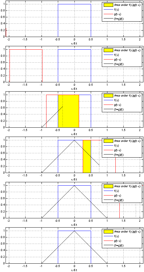
Read as: for each moment t, look back over all earlier moments \tau, take how strong the input was then, multiply by how much the system still responds after the elapsed time t-\tau, and add it all up.
The g(t-\tau) is the confusing part. The minus sign flips the response function around, which is why convolution is sometimes described as "flip and slide". It flips because \tau is measured forwards while the response is measured backwards from now.
The discrete version is what a computer runs, and it is easier to see:
(f*g)[n] = \sum_k f[k]\,g[n-k]
Worked example. Convolve [1,2,3] with [1,1].
Slide the second over the first and multiply-and-add at each offset:
- Position 0: 1\times1 = 1
- Position 1: 2\times1 + 1\times1 = 3
- Position 2: 3\times1+2\times1 = 5
- Position 3: 3\times1 = 3
Result: [1,3,5,3].
And you already knew this operation. Multiply the numbers 123 and 11 by hand:
123\times11 = 1353
The digits are exactly the convolution, because long multiplication is shifting and adding — which is the definition. Multiplication of polynomials is convolution of their coefficients, and multiplication of numbers is convolution of their digits with carrying. Chapter 8.5's generating functions rest on the same fact.
2. What it does, in three sentences
Convolution smooths. Convolving with a wide function spreads every feature out.
Convolution is what every linear time-invariant system does to its input. If a system's behaviour does not change over time and it treats a sum of inputs as the sum of their outputs, then its entire behaviour is captured by its impulse response, and its output is the input convolved with that response. Every filter, every echo, every lens blur, every circuit is described by one function.
Convolution is where blurring comes from. An out-of-focus camera convolves the true image with a small disc; camera shake convolves it with the path the camera travelled; the atmosphere convolves a star with a blob. In each case the recorded image is the truth convolved with something.
3. The convolution theorem
\widehat{f*g} = \hat f \cdot \hat g
Convolution in one domain is ordinary multiplication in the other.
This is the single most useful theorem in signal processing, for two reasons.
It explains what filtering is. A filter is defined by which frequencies it passes and which it blocks. In the frequency domain that is simple multiplication — multiply by 1 where you want to keep, by 0 where you want to remove. In the time domain the same operation is a convolution with the filter's impulse response. The two are the same operation seen from two sides, and the frequency side is the one that makes sense to a human.
It makes convolution fast. Direct convolution of two length-N signals costs N^2 operations. Transform both, multiply pointwise, transform back:
N\log N + N + N\log N = O(N\log N)
For N = 10^6 that is a fifty-thousand-fold saving, and it is why long reverbs, large image filters and big-number multiplication are computed this way rather than directly.
Convolution is commutative, which is not obvious from the definition and is immediate from the theorem — multiplication of the transforms obviously commutes, so the convolutions must too. Convolving the signal with the filter and the filter with the signal give identical results.
4. Filters
A filter modifies a signal's frequency content, and the four basic kinds are named by what they keep.
Low-pass keeps low frequencies, removes high. This is a blur or a smoother. In audio it muffles; in images it softens; in data it removes noise and leaves the trend.
High-pass keeps high frequencies. This is a sharpener or an edge detector, since edges are where values change fast.
Band-pass keeps a range. A radio tuner.
Notch removes a narrow range. Removing 50 Hz mains hum from a recording.
A moving average is a low-pass filter. Convolving with [\frac13,\frac13,\frac13] replaces each value with the average of three, which smooths.
A difference is a high-pass filter. Convolving with [-1,1] gives the change between consecutive samples, which is Chapter 5.2's derivative computed discretely, and it is large exactly where the signal changes fast.
There is always a trade-off. A filter with a sharp cut-off in frequency has a long impulse response in time, so it introduces delay and ringing (the Gibbs phenomenon of Chapter 9.2). A short, gentle filter is quick and imprecise. This is Chapter 9.3's uncertainty principle, arriving again as a practical engineering constraint.
5. Convolution in images
For a two-dimensional image, convolve with a small grid of numbers called a kernel. Each output pixel is a weighted sum of its neighbourhood.
Box blur — every weight equal. Simple and produces slight artefacts.
\frac19\begin{bmatrix}1&1&1\\1&1&1\\1&1&1\end{bmatrix}
Gaussian blur — weights following the bell curve of Chapter 7.6, heaviest at the centre. The standard blur everywhere, because the Gaussian's transform is another Gaussian, so it has no ringing at all.
Sharpen — subtract a blurred copy from the original, which removes the low frequencies and leaves the detail.
Sobel edge detection — a difference in one direction and a smoothing in the other:
\begin{bmatrix}-1&0&1\\-2&0&2\\-1&0&1\end{bmatrix}
This responds strongly to vertical edges and weakly to flat regions. The transposed version finds horizontal edges, and combining the two gives edge strength and direction.
Every filter in every image editor is one of these, and "kernel", "convolution" and "blur radius" in a photo application are literally this mathematics with a slider attached.
Convolutional neural networks
The CNN, which made computer vision work, is built on exactly this operation. Volume I, 12.4 covers the architecture.
The difference from a hand-designed filter is that the kernel weights are learned rather than chosen. Instead of someone deciding that [-1,0,1] detects edges, the network adjusts the numbers by gradient descent until they detect whatever is useful for the task.
Trained networks reliably learn edge and colour detectors in their first layer — very close to the Sobel kernels above — then texture detectors, then shapes, then objects. Nobody designed that hierarchy; it emerges because it is what the data rewards.
Two properties make convolution the right tool for images. The same kernel slides over the whole image, so a feature is detected wherever it appears — translation invariance. And a kernel has a handful of weights regardless of image size, so the parameter count stays small.
6. Convolution in probability
The distribution of a sum of two independent random variables is the convolution of their distributions.
f_{X+Y} = f_X * f_Y
Why. To get a total of z, you can have X = x and Y = z-x, for any x. Multiply the probabilities (independence) and add over all the ways. That is the convolution formula exactly.
Two dice. Each is uniform over 1 to 6. Convolve the two uniform distributions and you get the familiar triangular distribution peaking at 7 — because 7 has six ways to occur and 2 has one.
And this explains the central limit theorem. Adding more independent variables means convolving more distributions, and repeated convolution smooths towards a bell shape whatever you start from. Chapter 7.6 stated the theorem; this is the mechanism behind it. It also connects through the transform: convolution becomes multiplication, and the transform of a Gaussian is a Gaussian, which is the shape that is stable under the operation.
Every formula above, built from scratch
None of the results in this chapter are worth memorising, because each one can be rebuilt in under a minute from something simpler. What follows is that rebuilding, one result at a time, so the formula and the reason for it sit on the same page as the explanation that needed them.
Convolution
(f*g)(t) = \int_{-\infty}^{\infty}f(\tau)g(t-\tau)\,d\tau
Read it as a process. Flip g backwards, slide it along by t, multiply it against f point by point, and add up the result. Do that for every t and you have the convolution.
What it models. Every linear time-invariant system — one whose response does not change over time and where doubling the input doubles the output — turns its input into its output by convolution with a fixed function, the impulse response. That covers a filter, an amplifier, a room's echo, a camera lens blurring an image, and a moving average.
\text{output} = \text{input} * \text{impulse response}
The convolution theorem.
\widehat{f*g} = \hat f\cdot\hat g \qquad\text{and}\qquad \widehat{f\cdot g} = \frac{1}{2\pi}\hat f*\hat g
Why it is true. Take the transform of the convolution and swap the order of the two integrals:
\int\left[\int f(\tau)g(t-\tau)d\tau\right]e^{-i\omega t}dt = \int f(\tau)\left[\int g(t-\tau)e^{-i\omega t}dt\right]d\tau
The inner integral is the transform of g shifted by \tau, which by the time-shift property is e^{-i\omega\tau}\hat g(\omega). Pull the \hat g out, since it does not depend on \tau:
= \hat g(\omega)\int f(\tau)e^{-i\omega\tau}d\tau = \hat g(\omega)\hat f(\omega)
Why this is the most valuable fact in signal processing. Convolving two signals of length n directly costs about n^2 operations. Transforming both, multiplying point by point, and transforming back costs about n\log n using the fast Fourier transform. For n = 10^6 that is the difference between 10^{12} operations and 2\times10^7 — fifty thousand times faster. Every audio filter, every image blur, every large multiplication of huge numbers goes through this route.
7. Where this shows up in your life
Every photograph you take. Lens blur, sensor processing, and every filter you apply afterwards.
Every reverb and echo effect. Convolution reverb records a real space's impulse response and convolves your recording with it, so a vocal can be placed in a specific cathedral.
Every equaliser and every noise gate.
Every AI vision model. Convolutional layers.
Every moving average on a chart. A low-pass filter, whether the analyst calls it that or not.
Every seismograph, radar and sonar. Matched filtering correlates the received signal with the expected shape, which is convolution with a time-reversed template.
Every large multiplication your computer performs on big numbers, including the arbitrary-precision arithmetic in cryptography.
The Fourier transform handles signals that oscillate. It struggles with signals that grow, and with the transient behaviour engineers care about most. A close relative handles both, and it is the tool that solves every circuit and control system.