Appearance
4.4 — Determinants and Inverses
Chapter 4.2 showed that some matrices destroy information: they squash the whole plane onto a line, and no undoing is possible. Chapter 4.3 found out which ones by running elimination and watching for a zero row.
There is a single number that answers the question in advance, and it turns out to mean something geometrically rich. It is the determinant, and the plain statement is:
\textbf{The determinant is the factor by which a transformation multiplies area (or volume).}
1. What the determinant measures
Take the unit square with corners at (0,0), (1,0), (0,1) and (1,1) — area 1. Apply a matrix. The square becomes a parallelogram, since parallel lines stay parallel under a linear map.
The determinant is that parallelogram's area.
For \begin{bmatrix} 3 & 0 \\ 0 & 2\end{bmatrix}, the square is stretched to 3 wide and 2 tall. Area 6, determinant 6.
For a rotation, the square turns but keeps its size. Area 1, determinant 1.
For \begin{bmatrix} 1 & 2 \\ 2 & 4\end{bmatrix}, both basis vectors land on the same line, so the "parallelogram" is flat. Area 0, determinant 0 — and that is exactly the singular matrix of Chapter 4.2.
\det A = 0 \quad\Longleftrightarrow\quad \text{the transformation flattens space} \quad\Longleftrightarrow\quad \text{no inverse exists}

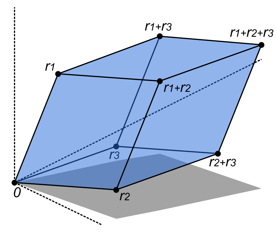
In three dimensions the unit cube becomes a slanted box (a parallelepiped), and the determinant is its volume. Zero means the cube got flattened into a plane, a line or a point.
2. A negative determinant means the space was flipped
Area cannot be negative, so what does \det = -1 mean?
It means orientation was reversed — the transformation includes a reflection. Before the transformation, going from the first basis vector to the second is an anticlockwise turn; afterwards it is clockwise. The space has been turned inside out.
A reflection \begin{bmatrix} 1 & 0\\0&-1\end{bmatrix} has determinant -1: same area, mirrored.
Where this matters concretely. In 3D graphics, a triangle facing you is drawn and one facing away is discarded, and the test is the sign of a determinant. Apply a transformation with negative determinant — a mirror — and every surface's facing flips, so a mirrored model renders inside out unless the winding order is corrected too. This is a real bug that shows up whenever someone scales a model by -1 on one axis to mirror it.
3. Computing determinants
Two by two:
\det\begin{bmatrix} a & b \\ c& d\end{bmatrix} = ad - bc
Check the flat case: \begin{bmatrix} 1&2\\2&4\end{bmatrix} gives 4 - 4 = 0. Correct.
Three by three, expanding along the top row:
\det\begin{bmatrix} a&b&c\\d&e&f\\g&h&i\end{bmatrix} = a(ei-fh) - b(di - fg) + c(dh - eg)
Each term is an entry times the determinant of the 2\times2 matrix left after deleting that entry's row and column — its minor — with signs alternating +, -, +.
Worked example.
\det\begin{bmatrix} 2&1&-1\\-3&-1&2\\-2&1&2\end{bmatrix} = 2\big((-1)(2)-(2)(1)\big) - 1\big((-3)(2)-(2)(-2)\big) + (-1)\big((-3)(1)-(-1)(-2)\big)
= 2(-4) - 1(-2) + (-1)(-5) = -8 + 2 + 5 = -1
Nonzero, so the system of Chapter 4.3 had a unique solution — which it did.
Larger than three by three: do not expand. The expansion method costs about n! operations, and 20! is 2.4 \times 10^{18} — longer than the age of the universe on any computer. Instead, run Gaussian elimination from Chapter 4.3 to triangular form and multiply the diagonal, which costs only n^3 operations. Row swaps flip the sign, and scaling a row scales the determinant, so keep track of those.
4. The rules the determinant obeys
\det(AB) = \det(A)\det(B)
The reason is obvious once you know what the determinant measures. If B multiplies area by 3 and A multiplies it by 5, doing both multiplies it by 15. The algebra follows from the geometry, not the other way round.
\det(A^\mathsf{T}) = \det(A) \qquad \det(A^{-1}) = \frac{1}{\det A} \qquad \det(cA) = c^n \det(A)
That last one catches people. Scaling a matrix by c scales every dimension by c, so in n dimensions the volume scales by c^n. Doubling every entry of a 3\times3 matrix multiplies the determinant by eight.
5. The inverse
The inverse A^{-1} undoes A:
AA^{-1} = A^{-1}A = I
If A rotates by 30°, its inverse rotates by -30°. If A doubles everything, its inverse halves it.
Only square matrices can have inverses, and only when \det A \neq 0. The geometric reason is the whole of Section 1: a flattening cannot be undone, because too much arrived at the same place.
For a 2\times2 matrix there is a formula:
A^{-1} = \frac{1}{ad-bc}\begin{bmatrix} d & -b \\ -c & a\end{bmatrix}
Swap the diagonal, negate the off-diagonal, divide by the determinant. The division makes the failure at \det = 0 visible — you would be dividing by zero, which Chapter 1.2 settled has no meaning.
Worked check. For A = \begin{bmatrix}2&1\\1&1\end{bmatrix}, \det = 1, so A^{-1} = \begin{bmatrix}1&-1\\-1&2\end{bmatrix}. Multiply:
\begin{bmatrix}2&1\\1&1\end{bmatrix}\begin{bmatrix}1&-1\\-1&2\end{bmatrix} = \begin{bmatrix}2-1 & -2+2\\1-1&-1+2\end{bmatrix} = \begin{bmatrix}1&0\\0&1\end{bmatrix} \;✓
A rule with a reversal in it: (AB)^{-1} = B^{-1}A^{-1}. Undoing "socks then shoes" means removing shoes first. The order reverses, exactly as with the transpose in Chapter 4.2.
Never compute an inverse to solve a system
It is tempting to write \mathbf{x} = A^{-1}\mathbf{b} and have a computer form A^{-1}. Do not.
Forming the inverse costs about three times as much work as elimination, and it is numerically worse — each entry of the inverse accumulates its own rounding error, and multiplying by it spreads that error into every component of the answer. Every numerical library therefore offers solve(A, b) rather than encouraging inv(A) @ b.
The inverse is a fine idea to think with and a bad thing to compute. That distinction — a concept that is essential for reasoning and wrong to implement literally — comes up repeatedly in numerical work, and Chapter 10.1 has more of it.
6. Cramer's rule, and its honest assessment
There is a formula that gives each unknown directly as a ratio of determinants:
x_i = \frac{\det(A_i)}{\det(A)}
where A_i is A with its $i$th column replaced by \mathbf{b}.
Worked example. For \begin{cases}2x + y = 5\\ x + 3y = 10\end{cases}:
\det A = 6 - 1 = 5, \qquad \det A_1 = \det\begin{bmatrix}5&1\\10&3\end{bmatrix} = 5, \qquad \det A_2 = \det\begin{bmatrix}2&5\\1&10\end{bmatrix} = 15
So x = 1 and y = 3. Check: 2+3 = 5 ✓, 1 + 9 = 10 ✓.
It is elegant, and it is essentially never used computationally — it needs n+1 determinants, which is far more work than one elimination. Its value is theoretical: it proves that when \det A \neq 0 a unique solution exists and is a smooth function of the inputs, which matters for proofs and for understanding sensitivity. Know it exists, do not implement it.
7. The trace, and a preview
One more number attached to a square matrix: the trace, the sum of the diagonal entries.
\operatorname{tr}\begin{bmatrix} 2&1\\3&4\end{bmatrix} = 6
It has a surprising property: \operatorname{tr}(AB) = \operatorname{tr}(BA), even though AB \neq BA in general.
Trace and determinant matter together because they are the two quantities that survive a change of coordinate system. Describe the same transformation in a different basis and every entry of the matrix changes — but the determinant and the trace do not. They are properties of the transformation, not of the numbers you happened to write down.
Chapter 4.5 explains why: the determinant is the product of the eigenvalues and the trace is their sum, and eigenvalues belong to the transformation itself.
Every formula above, built from scratch
None of the results in this chapter are worth memorising, because each one can be rebuilt in under a minute from something simpler. What follows is that rebuilding, one result at a time, so the formula and the reason for it sit on the same page as the explanation that needed them.
Determinants
\det\begin{pmatrix}a&b\\c&d\end{pmatrix} = ad-bc
Where it comes from. The determinant is the factor by which areas are multiplied. Take the unit square, whose corners are (0,0), (1,0), (1,1), (0,1), with area 1. After the matrix acts, it becomes a parallelogram with sides (a,c) and (b,d). The area of a parallelogram spanned by two plane vectors is |u_1v_2 - u_2v_1|, which for our two columns is |ad-cb|. So the square of area 1 became a shape of area |ad-bc|, and every other region scales by the same factor since the transformation treats all of space alike.
Why the sign matters. A negative determinant means the plane was flipped over — the transformation turned the shape into its mirror image, as reflecting in an axis does. The size of the number is the area factor; the sign is the orientation.
\det = 0 means the transformation crushed space. The two columns lie on the same line, the unit square is flattened into a segment of zero area, and information is destroyed. That single fact is why a zero determinant means "no inverse": you cannot undo a collapse, because many different starting points all landed on the same place.
Three by three
\det\begin{pmatrix}a&b&c\\d&e&f\\g&h&i\end{pmatrix} = a(ei-fh) - b(di-fg) + c(dh-eg)
This is expansion along the first row: take each entry, multiply by the determinant of the 2\times2 left after deleting its row and column, and alternate the signs +,-,+. In three dimensions the determinant is the volume scaling factor, and the alternating signs come from orientation flipping each time you step across.
You may expand along any row or column, and choosing one with zeros in it saves most of the work.
The properties that make determinants usable
\det(AB) = \det A\det B, \qquad \det(A^T) = \det A, \qquad \det(A^{-1}) = \frac{1}{\det A}, \qquad \det(cA) = c^n\det A
Why \det(AB) = \det A\det B needs no calculation. Apply B, which multiplies areas by \det B. Then apply A, which multiplies areas by \det A. Doing both multiplies areas by the product. Since AB is the single transformation that does both, its area factor is that product.
Why \det(cA) = c^n\det A. Scaling every entry by c stretches all n dimensions by c, and volume in n dimensions scales by c^n.
Row operations. Swapping two rows flips the sign. Adding a multiple of one row to another leaves it unchanged. Multiplying a row by k multiplies it by k. These three rules are what make Gaussian elimination the practical way to compute a determinant: reduce to triangular form, where the determinant is just the product down the diagonal.
Inverses
A^{-1} = \frac{1}{ad-bc}\begin{pmatrix}d & -b\\ -c & a\end{pmatrix} \qquad \text{for } A = \begin{pmatrix}a&b\\c&d\end{pmatrix}
Where it comes from. We want A^{-1} with AA^{-1} = I. Write the unknown as \begin{pmatrix}p&q\\r&s\end{pmatrix} and multiply out:
\begin{pmatrix}a&b\\c&d\end{pmatrix}\begin{pmatrix}p&q\\r&s\end{pmatrix} = \begin{pmatrix}ap+br & aq+bs\\ cp+dr & cq+ds\end{pmatrix} = \begin{pmatrix}1&0\\0&1\end{pmatrix}
That gives four equations. From the first column, ap+br = 1 and cp+dr = 0. The second gives r = -\frac{cp}{d}; substituting into the first:
ap - \frac{bcp}{d} = 1 \quad \Rightarrow \quad p\frac{ad-bc}{d} = 1 \quad \Rightarrow \quad p = \frac{d}{ad-bc}
and then r = \frac{-c}{ad-bc}. The second column works the same way and gives q = \frac{-b}{ad-bc}, s = \frac{a}{ad-bc}. Collecting them produces the formula: swap the diagonal, negate the off-diagonal, divide by the determinant.
The division by ad-bc is where "no inverse when the determinant is zero" comes from — not as a rule to remember but as a division by zero you can see.
The general version.
A^{-1} = \frac{1}{\det A}\operatorname{adj}(A)
where the adjugate is the transpose of the matrix of cofactors. It is beautiful and almost never used for computation: for a 10\times10 matrix it needs millions of times more arithmetic than elimination. Real software solves A\mathbf{x} = \mathbf{b} by elimination and never forms A^{-1} at all.
Cramer's rule
x_i = \frac{\det A_i}{\det A}
where A_i is A with its i-th column replaced by \mathbf{b}.
Why it works. Solving A\mathbf{x}=\mathbf{b} means finding the combination of A's columns that produces \mathbf{b}. Replacing column i by \mathbf{b} and taking the determinant measures how much of the total "volume" is contributed by that column's coefficient, and dividing by the whole volume isolates it. It is elegant, it proves the solution is unique when \det A\ne0, and for anything larger than 3\times3 it is far too slow to use.
8. Where this shows up in your life
Every 3D graphics pipeline. Determinant sign decides which faces to draw and which to discard.
Every calculus change of variables. When you switch from Cartesian to polar coordinates in an integral, the extra factor of r that appears is a determinant — the Jacobian — measuring how much the coordinate change stretches area. Chapter 5.7 covers it.
Every check for redundant data. A determinant of zero (or very near zero) in a data matrix means your columns are dependent and your model is about to behave unpredictably.
Every stability analysis in engineering. Whether a bridge, an aircraft or a control loop is stable depends on determinants of the system matrix, via the eigenvalues of the next chapter.
Every area calculation from coordinates. A surveyor's plot with corners at known coordinates has its area computed by the shoelace formula, which is a sum of 2\times2 determinants.
The determinant tells you the total stretching. It does not tell you the directions in which the stretching happens, and those directions turn out to be the deepest thing about a matrix.