Appearance
6.4 — Partial Differential Equations
Heat one end of an iron bar. The temperature is now different at every point and at every moment — it is a function of both position and time, T(x,t).
An equation describing this must involve how the temperature changes with time and how it varies through space. That means partial derivatives from Chapter 5.7, and an equation containing them is a partial differential equation, a PDE.
Three of them describe an enormous fraction of physics, and they are worth knowing by sight because you will meet them repeatedly.
1. The heat equation
\frac{\partial T}{\partial t} = \alpha\frac{\partial^2 T}{\partial x^2}
Read it in plain words: the temperature at a point rises when that point is colder than the average of its neighbours.
Here is why the second derivative says that. Chapter 5.2 explained that \frac{\partial^2 T}{\partial x^2} measures concavity. If the temperature profile is curved upward at a point — a dip — then the neighbours on both sides are hotter, so heat flows in and the temperature rises. If it is curved downward — a bump — the neighbours are colder, heat flows out, and it falls.
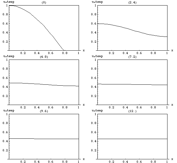
The equation is therefore a statement about smoothing. Bumps get flattened, dips get filled, and everything drifts towards uniformity. Anyone who has watched a hot spot spread and fade has watched this equation run.
The constant \alpha is the thermal diffusivity and it sets the speed. Copper's is high, so heat races through it; wood's is low, which is why a wooden spoon in hot soup stays cool at the handle.
Two properties worth noticing.
It smooths instantly. Even a starting profile with a sharp corner becomes perfectly smooth the instant after t=0. Sharp features are destroyed first.
It cannot be run backwards. Given today's temperature you can compute tomorrow's; given today's you cannot reliably reconstruct yesterday's, because the information in the sharp features has already been destroyed. This is one of the few places where mathematics contains an arrow of time, and it is connected to entropy — Volume IV, Chapter 3.
The same equation governs diffusion of anything. Replace temperature with concentration and it describes a drop of ink spreading in water, a smell filling a room, a drug distributing through tissue, or a pollutant in groundwater. Replace it with probability and it describes Brownian motion, the random walk of a particle. Replace it with option price and it is the Black–Scholes equation of mathematical finance, which is the heat equation after a change of variables.
And it is why image blurring works the way it does. Running the heat equation on an image blurs it, since it averages each pixel towards its neighbours. Running it backwards would sharpen — which is exactly why sharpening amplifies noise and cannot recover genuinely lost detail.
2. The wave equation
\frac{\partial^2 u}{\partial t^2} = c^2\frac{\partial^2 u}{\partial x^2}
Almost the same, with one change: the time derivative is now second order.
That single change transforms the behaviour completely. In the heat equation, curvature drives velocity, so things drift towards flat and stop. Here curvature drives acceleration, so the string overshoots the flat position and keeps going — exactly the difference between Chapter 6.1 and Chapter 6.2, now in space as well as time.
The result is not smoothing but travelling and oscillation. D'Alembert showed in 1747 that every solution has the form
u(x,t) = f(x - ct) + g(x + ct)
Two shapes, one moving right at speed c and one moving left, keeping their form as they go. The constant c is the wave speed, and it comes from the physical properties: for a string, c = \sqrt{T/\mu} with T the tension and \mu the mass per unit length. Tighten a guitar string and the wave travels faster, so the pitch rises. Use a thicker string and it travels slower, so the pitch drops. That is the whole physics of tuning a guitar, in one formula.
Standing waves. Fix both ends of a string and only certain wavelengths fit — those with a whole number of half-waves between the ends. These are the harmonics, and their frequencies are whole-number multiples of the lowest one.
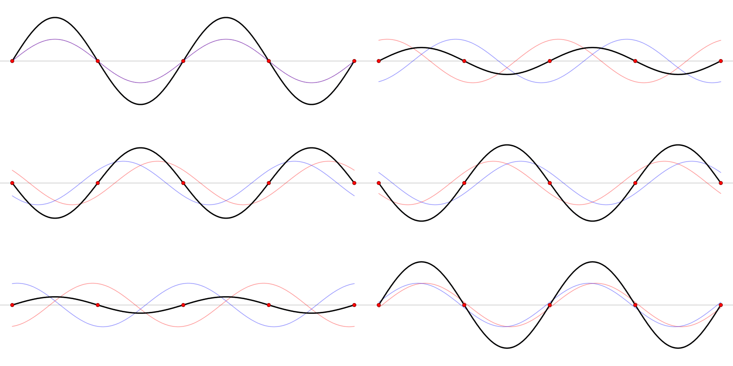
This is why musical instruments have pitch at all, and why a note from a violin and the same note from a flute sound different: they are the same fundamental frequency with different mixtures of harmonics. That mixture is the timbre, and Chapter 9.2 shows how to extract it.
Everything that propagates obeys this equation: sound in air, light and radio in space (which is what Maxwell's equations reduce to), ripples on water, seismic waves through rock, and the vibration of every structure.
3. Laplace's equation
Set the time derivative to zero in the heat equation — the steady state, after everything has settled:
\frac{\partial^2 u}{\partial x^2}+\frac{\partial^2 u}{\partial y^2} = 0, \qquad\text{written}\qquad \nabla^2 u = 0
Read it as: every point's value is exactly the average of its neighbours. No point is a bump or a dip.
Solutions are called harmonic functions, and they have two remarkable properties.
The maximum principle. A harmonic function's largest and smallest values are always on the boundary, never inside. There are no interior peaks — a peak would be above its neighbours' average, which the equation forbids. So the temperature inside a metal plate at steady state is never hotter than the hottest edge, which is intuitively obvious and now provable.
The boundary determines everything. Fix the values on the boundary and the interior is completely determined. There is one and only one solution. This is why "solve for the field inside, given the conditions on the surface" is a well-posed engineering question.
Where it appears: steady temperature distributions, the electric potential in charge-free space, gravitational potential, the flow of an ideal fluid, the shape of a soap film stretched on a wire loop (it minimises area, which forces this equation), and the steady seepage of groundwater.
4. Solving PDEs: separation of variables
The classical technique. Guess that the solution is a product of single-variable functions:
u(x,t) = X(x)\,T(t)
Substitute into the heat equation and divide through by XT:
\frac{T'}{\alpha T} = \frac{X''}{X}
The left side depends only on t and the right only on x. The only way a function of t can equal a function of x for all values of both is if both are the same constant. Call it -\lambda. Now there are two ordinary differential equations, and Chapters 6.1 and 6.2 already solve both:
T' = -\alpha\lambda T \;\Rightarrow\; T = e^{-\alpha\lambda t}, \qquad X'' = -\lambda X \;\Rightarrow\; X = \sin(\sqrt\lambda x) \text{ or } \cos(\sqrt\lambda x)
The boundary conditions pick out which values of \lambda are allowed — for a bar of length L held at zero at both ends, \sqrt\lambda = \frac{n\pi}{L} for whole numbers n.
Then add them all up. Because the equation is linear, any sum of solutions is a solution:
u(x,t) = \sum_{n=1}^{\infty}b_n\sin\!\left(\frac{n\pi x}{L}\right)e^{-\alpha(n\pi/L)^2 t}
The coefficients b_n are fixed by matching the initial temperature profile at t=0 — which means writing an arbitrary starting shape as a sum of sines.
And that is precisely the problem Fourier solved. He was working on heat conduction, needed to express an arbitrary function as a sum of sines, claimed it could always be done, and was disbelieved by the leading mathematicians of the day. Chapter 9.2 tells the story and does the mathematics. Fourier analysis was invented to solve this equation, and it went on to become the foundation of signal processing.
Notice one thing in that solution. The exponential factor contains n^2, so high-frequency components (n large) decay dramatically faster than low-frequency ones. That is the mathematical statement of "sharp features vanish first" — sharpness lives in the high harmonics, and the heat equation kills them fastest. The same fact is why a low-pass filter blurs an image.
5. What is hard about PDEs
Ordinary differential equations are, in general, solvable numerically without drama. PDEs are a different world.
Most have no closed-form solution. The methods above work for simple geometries — a straight bar, a rectangle, a circle. Real problems have complicated shapes, and then you compute numerically.
Numerical methods are their own discipline. Finite differences replace derivatives with difference quotients on a grid. The finite element method breaks the region into small triangles or tetrahedra and solves on each. Every structural analysis, crash simulation, aerodynamic calculation and electromagnetic design tool is a finite element solver, and each is ultimately assembling and solving an enormous sparse linear system — Chapter 4.3's Gaussian elimination, at scale.
Stability is a real constraint. A time-stepping scheme for the heat equation is unstable unless the time step is small enough relative to the grid spacing — specifically, the step must shrink with the square of the grid spacing. Halve the grid and you must quarter the time step, so refining a simulation is far more expensive than it looks. Chapter 10.3 covers this.
And one is worth a million dollars. The Navier–Stokes equations describe fluid flow, and they are used every day for aircraft, weather, blood flow and ocean currents. Nobody has proved that smooth solutions always exist in three dimensions, or found a case where one breaks down. It is one of the seven Millennium Prize Problems, and Chapter 11.4 discusses them. We simulate fluids constantly without knowing whether the equations always behave.
Every formula above, built from scratch
None of the results in this chapter are worth memorising, because each one can be rebuilt in under a minute from something simpler. What follows is that rebuilding, one result at a time, so the formula and the reason for it sit on the same page as the explanation that needed them.
Partial differential equations
\text{Heat: } \frac{\partial u}{\partial t} = \alpha\frac{\partial^2u}{\partial x^2}, \qquad \text{Wave: } \frac{\partial^2u}{\partial t^2} = c^2\frac{\partial^2u}{\partial x^2}, \qquad \text{Laplace: } \nabla^2u = 0
What each one says. The heat equation: temperature rises where the profile is curved upwards, that is, where a point is colder than the average of its neighbours. The wave equation: acceleration is proportional to curvature, so a taut string pulls itself back towards straightness. Laplace's equation: the steady state after everything has settled, where every point is exactly the average of its surroundings.
Separation of variables, the standard method. Assume the solution factorises, u(x,t) = X(x)T(t), and substitute. For the heat equation:
XT' = \alpha X''T \quad \Rightarrow \quad \frac{T'}{\alpha T} = \frac{X''}{X}
The left side depends only on t; the right only on x. Two expressions in different variables can be equal for all values only if both are the same constant, call it -\lambda. The single partial differential equation has split into two ordinary ones:
T' = -\alpha\lambda T, \qquad X'' = -\lambda X
Both are from §2 and §6. The boundary conditions then pick out which values of \lambda are allowed, and adding up all the allowed solutions gives a Fourier series — which is exactly why Part 9 exists, and exactly the problem Fourier was working on when he invented it.
D'Alembert's solution of the wave equation:
u(x,t) = f(x-ct)+g(x+ct)
Any shape moving right at speed c, plus any shape moving left at speed c. Substituting confirms it, and it explains everything about echoes, reflections and the fact that a wave carries its shape along unchanged.
6. Where this shows up in your life
Every weather forecast. The atmosphere is Navier–Stokes plus thermodynamics on a rotating sphere, solved numerically on a grid.
Every engineering simulation. Stress in a bracket, heat in a processor, airflow over a wing, the crumple of a car in a crash.
Every medical scan. MRI reconstruction and ultrasound both rest on wave propagation.
Every image blur, sharpen and denoise operation. The heat equation, forwards and backwards.
Every noise-cancelling headphone. Wave superposition, and the fact that the wave equation is linear so two waves can cancel.
Every option priced in a bank. Black–Scholes is the heat equation wearing financial clothes.
Every building's thermal design and every heatsink in your computer. Steady-state heat conduction, which is Laplace's equation.
Part 6 is finished. The equations of change are in place. What we have not touched is uncertainty — everything so far has been exact, and most of the world is not. That is probability, and it is the other half of applied mathematics.
More places these turn up
Newton's cooling law sets the timer on your fridge and the estimate on a coroner's report. The logistic curve was on every news broadcast during an epidemic, and it is the shape of every product's adoption. Critical damping is why your car does not bounce and why a screen door does not slam. Resonance is why a bridge has dampers, why a helicopter has a rotor speed it must pass through quickly, and why an MRI scanner is called magnetic resonance imaging. The heat equation prices financial options after a change of variables, and it smooths the noise out of every photograph your phone takes.
Next: 6.P — Worked Problems solves each type in full, from separable equations to a damped spring with a driving force.