Appearance
6.3 — Systems, Stability and Chaos
Foxes eat rabbits. More rabbits mean more food, so the fox population grows. More foxes mean fewer rabbits. Fewer rabbits mean the foxes starve, so their numbers fall. Fewer foxes mean the rabbits recover.
Neither population can be described on its own — each one's rate of change depends on the other. That needs two equations solved together, and once you have coupled equations, entirely new behaviour becomes possible: cycles, spirals, tipping points, and eventually unpredictability that no amount of better measurement can remove.
1. Systems of differential equations
\begin{cases}\dfrac{dx}{dt} = f(x,y) \\[6pt] \dfrac{dy}{dt} = g(x,y)\end{cases}
The Lotka–Volterra predator–prey model, from the 1920s:
\frac{dR}{dt} = aR - bRF, \qquad \frac{dF}{dt} = cRF - dF
Read each term as a sentence. Rabbits breed in proportion to their number (aR) and are eaten at a rate proportional to how often the two species meet, which is proportional to the product (bRF). Foxes die off at a steady rate (dF) and are born in proportion to how much they eat (cRF).
The RF terms make it nonlinear, and they are also what makes it interesting — the interaction is the whole model.
The solutions cycle. Rabbits rise, foxes follow, rabbits crash, foxes crash, rabbits recover. The fox peak always lags the rabbit peak by a quarter cycle. Hudson's Bay Company fur-trapping records for lynx and snowshoe hare, going back to the 1840s, show exactly this pattern with a roughly ten-year period.
The counterintuitive result that cost fishermen money
Add a term for harvesting both species — fishing, in the original case Volterra was studying. Work through the equilibrium and you find something strange: harvesting both predator and prey increases the average number of prey and decreases the average number of predators.
Volterra was asked to explain why, during the First World War when Adriatic fishing largely stopped, the proportion of sharks in the catch went up. The model said it should: less fishing means more predators. It is now called Volterra's principle, and it is the reason a broad-spectrum pesticide can make a pest problem worse — it kills the pest's predators along with the pest, and the pest rebounds faster.
2. The phase plane
Rather than plotting x and y against time separately, plot y against x and let time be implicit. Each solution becomes a curve — a trajectory — and the whole picture is the phase portrait.
For the predator–prey system the trajectories are closed loops, going round and round, which is exactly what a repeating cycle looks like in this view.
This is where the real understanding lives. You can read off every possible long-term behaviour from the shape of the picture without solving anything.
Equilibrium points are where both rates are zero — the system sits still. Their types:
- Stable node: everything nearby flows in. A ball at the bottom of a bowl.
- Unstable node: everything flows out. A ball on top of a dome.
- Saddle: flows in along one direction and out along another. A ball on a mountain pass — stable if it stays exactly on the ridge, unstable to any sideways nudge.
- Centre: closed loops around it. The predator–prey case.
- Spiral: spirals in (stable) or out (unstable). A damped oscillation from Chapter 6.2 is a stable spiral.
Classifying them is linear algebra. Near an equilibrium, replace the system by its linear approximation — the matrix of partial derivatives, called the Jacobian — and look at its eigenvalues (Chapter 4.5):
| Eigenvalues | Type |
|---|---|
| both real negative | stable node |
| both real positive | unstable node |
| real, opposite signs | saddle |
| complex, negative real part | stable spiral |
| complex, positive real part | unstable spiral |
| purely imaginary | centre |
The rule in one line: negative real parts mean stable, positive means unstable, and an imaginary part means rotation. That single sentence is used by every control engineer, every ecologist and every economist who models a dynamic system.
3. Chaos
Now something that overturned a three-hundred-year assumption.
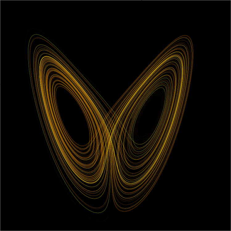
In 1961 Edward Lorenz was running a simplified weather model on an early computer. Restarting a run partway through, he typed in the numbers from a printout — which showed six digits where the machine held twelve. He expected a slightly different result. He got a completely different weather.
His equations:
\dot x = \sigma(y-x), \qquad \dot y = x(\rho - z) - y, \qquad \dot z = xy - \beta z
Three variables, no randomness whatsoever, entirely determined by the starting values. And yet two starting points differing in the sixth decimal place diverge to entirely different outcomes within a modest span of simulated time.
This is chaos: deterministic, and unpredictable.
Three features define chaos.
Sensitive dependence on initial conditions. Two nearby starts separate exponentially. This is the butterfly effect, from the title of Lorenz's 1972 talk asking whether a butterfly's wings in Brazil could set off a tornado in Texas. Note what it does not claim — that the butterfly caused the tornado — but that in a chaotic system, an unmeasurably small difference eventually matters.
Topological mixing. Any small patch of starting points eventually spreads out over the whole attractor.
Dense periodic orbits. Arbitrarily close to any point there is a repeating trajectory, so the structure is threaded with periodicity while the motion never actually repeats.
Why this matters for weather. Chaos sets a hard limit. Weather forecasts are good for about three days, useful to a week, and worthless beyond about two weeks — and no improvement in computers or models will change that. The limit is not our ignorance; it is the equations. To forecast a month ahead you would need initial measurements accurate to more decimal places than physically exist.
Modern forecasting responds honestly: run the model many times from slightly perturbed starting points — an ensemble — and report how many runs agree. "70% chance of rain" is literally the fraction of ensemble members that produced rain.
Climate is different from weather, and the distinction is exactly this. You cannot say whether it will rain in Kolkata on 3 August next year, and you can say what the average August rainfall will be. Chaos scrambles trajectories while leaving statistics stable — the Lorenz trajectory is unpredictable, and the attractor's shape is completely fixed.
4. The logistic map: chaos with one line of arithmetic
Chaos does not need three dimensions or differential equations. Take the simplest nonlinear recurrence:
x_{n+1} = rx_n(1-x_n)
the discrete version of Chapter 6.1's logistic growth. Vary r and watch.
- r \lt 3: settles to one value.
- r \approx 3.2: settles into alternating between two values. A period doubling.
- r \approx 3.5: four values.
- Then 8, 16, 32, with the doublings arriving faster and faster.
- r \approx 3.57: the doublings have accumulated, and the behaviour becomes chaotic — never repeating.
- Above that: chaos, with narrow windows of order embedded in it, including a clearly visible period-3 window.

And now the astonishing part. Mitchell Feigenbaum measured the ratio of successive doubling intervals in 1975 and found it approaches a constant:
\delta = 4.669201609\ldots
The same constant appears for every system that reaches chaos by period doubling — a dripping tap, an oscillating chemical reaction, a heart arrhythmia, a laser, a convecting fluid. It does not matter what the system is made of. This is universality, and it means chaos has a mathematical structure of its own, independent of physics.
5. Attractors and fractals
An attractor is the set a system settles onto in the long run.
- A fixed point — the damped pendulum comes to rest.
- A limit cycle — a repeating loop. A heartbeat, a firefly's flashing, a self-sustaining oscillator.
- A strange attractor — the chaotic case, and it is a fractal in the sense of Chapter 3.6, with a non-integer dimension. The Lorenz attractor's dimension is about 2.06: more than a surface, less than a solid.
The trajectory is confined to the attractor forever and never repeats a point on it. That combination — bounded and never repeating — requires infinite intricacy, which is precisely why the attractor must be a fractal.
A double pendulum — one pendulum hanging from another — is the simplest mechanical system that is chaotic, and you can build one from two rulers and a bolt. Release it twice from as close to the same position as you can manage and the two motions diverge within seconds.

6. What chaos changed about the world
Laplace wrote in 1814 that an intellect knowing every particle's position and velocity could compute the entire future. That was the confident view for two centuries: determinism means predictability.
Chaos separated the two. A system can be perfectly deterministic and practically unpredictable, and no better instrument fixes it, because the required precision grows exponentially with the forecast horizon.
That is a genuinely different kind of limit from the ones in Chapter 1.7 or Volume I, 1.7 — it is not that the answer is unknowable in principle, but that knowing it would require infinite precision in the input.
Where the idea is now used:
- Cardiology. A healthy heartbeat has some chaotic variability; too regular a rhythm can be a warning sign.
- Ecology. Population crashes can arise from the internal dynamics alone, with no external cause to find.
- Engineering. Chaos control adds tiny, well-timed nudges to stabilise a chaotic system onto one of its embedded periodic orbits — used to stabilise lasers and, experimentally, cardiac rhythms.
- Cryptography and simulation. Sensitive dependence makes chaotic maps useful for mixing, though the pseudo-random generators of Volume I, 8.2 remain the right tool for anything security-related.
- Economics. Business cycles and market crashes may be internal dynamics rather than responses to news, which is a genuinely unsettling possibility for forecasting.
Every formula above, built from scratch
None of the results in this chapter are worth memorising, because each one can be rebuilt in under a minute from something simpler. What follows is that rebuilding, one result at a time, so the formula and the reason for it sit on the same page as the explanation that needed them.
Systems and the phase plane
\dot{\mathbf{x}} = A\mathbf{x} \quad \Rightarrow \quad \mathbf{x}(t) = c_1e^{\lambda_1t}\mathbf{v}_1 + c_2e^{\lambda_2t}\mathbf{v}_2
where the \lambda's and \mathbf{v}'s are the eigenvalues and eigenvectors of 4.5 — eigenvalues.
Why this is the answer. Try \mathbf{x} = e^{\lambda t}\mathbf{v} for a constant vector \mathbf{v}. Then \dot{\mathbf{x}} = \lambda e^{\lambda t}\mathbf{v}, and the equation becomes
\lambda e^{\lambda t}\mathbf{v} = Ae^{\lambda t}\mathbf{v} \quad \Rightarrow \quad A\mathbf{v} = \lambda\mathbf{v}
which is exactly the eigenvalue equation. The eigenvectors are the directions along which the system evolves by simple scaling, and every other motion is a combination of them.
The classification of behaviour, entirely from the eigenvalues:
| Eigenvalues | Picture | Stability |
|---|---|---|
| both real, negative | node | stable |
| both real, positive | node | unstable |
| real, opposite signs | saddle | unstable |
| complex, negative real part | spiral inwards | stable |
| complex, positive real part | spiral outwards | unstable |
| purely imaginary | closed loops | neutral |
The one rule underneath the table: the real part decides whether things grow or shrink, and the imaginary part decides whether they rotate.
Nonlinear systems are handled by linearising near each equilibrium point — replace the system by its Jacobian matrix of partial derivatives — and reading the table above. That works everywhere except the borderline cases, and it is where chaos hides.
7. Where this shows up in your life
Every weather forecast, including why it comes with a percentage and why it stops being useful after a week.
Every climate discussion. Knowing why weather is unpredictable and climate is not is the single most useful thing this chapter gives you for public conversation.
Every ecological or epidemic model. Coupled populations, phase portraits, stability of equilibria.
Every control system's stability analysis. Eigenvalues with negative real parts, Section 2.
Every double-jointed toy, every dripping tap, every swirl of cream in coffee. All chaotic, all describable, none predictable.
Everything so far has changed with time alone. When something varies across space as well — heat spreading through metal, a wave running along a string, a field filling a region — you need partial derivatives, and the equations that result are the ones physics is actually written in.