Appearance
7.8 — Hypothesis Testing and Regression
A new website design converts 12% of visitors; the old one converted 10%. Is the new design better, or did you just get a lucky sample?
That question — real effect or noise? — is asked constantly in medicine, science, business and engineering. Answering it is hypothesis testing, and it is simultaneously the most widely used and most widely misused tool in statistics.
1. The logic
Assume nothing is happening. Then ask how surprising your data would be.
The null hypothesis H_0 is the boring claim: no difference, no effect, no relationship. The alternative hypothesis H_1 is what you suspect.
The procedure:
- Assume H_0 is true.
- Compute how likely data as extreme as yours would be under that assumption. That is the p-value.
- If the p-value is small, the data is hard to reconcile with H_0, so reject it.
- If not, you have failed to reject H_0 — which is not the same as proving it.
The asymmetry matters. This is a proof by contradiction (Chapter 1.7) with probability in place of certainty. You can gather evidence against the null; you cannot gather evidence for it in this framework. "Not significant" means "we did not see enough to rule out chance", not "there is no effect".
What a p-value is, and what it is not
p = P(\text{data this extreme}\mid H_0 \text{ true})
It is not P(H_0\text{ true}\mid\text{data}). Those two are related by Bayes' theorem (Chapter 7.3), and swapping them is the same prosecutor's fallacy that sent Sally Clark to prison.
A p-value of 0.03 does not mean a 3% chance the null is true. It means: if the null were true, you would see data this extreme 3% of the time.
To get the probability the null is true you would need a prior, and the p-value framework deliberately does not have one. This single confusion is responsible for more misreported science than any other error in statistics.

2. The two errors
| H_0 true | H_0 false | |
|---|---|---|
| Reject H_0 | Type I error (false positive) | correct |
| Fail to reject | correct | Type II error (false negative) |
Type I: you announce an effect that is not there. Its probability is \alpha, the significance threshold you chose.
Type II: you miss an effect that is there. Its probability is \beta, and 1-\beta is the power of the test.
The two trade off. Demanding stronger evidence (smaller \alpha) means missing more real effects. Which error is worse depends entirely on the situation: a cancer screening test should tolerate false positives to avoid false negatives; a criminal trial is deliberately built the other way, on the principle that convicting the innocent is worse than acquitting the guilty.
Power depends on sample size. An underpowered study — too few participants — will miss real effects, and a great deal of published research is underpowered. Power should be calculated before running the study, not after, and a study that could never have detected the effect it was looking for was not worth running.
3. The 0.05 problem
The threshold \alpha = 0.05 has no principled basis whatsoever. Ronald Fisher suggested it in 1925 as a convenient rule of thumb and later said explicitly that no fixed level should be used for all cases.
It became a bright line anyway, and the consequences have been serious.
Publication bias. Journals publish significant results. A drawer full of non-significant studies never appears, so the published literature is a biased sample of all studies conducted. If twenty teams test a null effect, one will get p \lt 0.05 by chance, and that one gets published.
p-hacking. Try many analyses, report the one that crosses 0.05. Drop outliers, add covariates, split subgroups, test several outcomes, stop collecting data when the result looks good. Each choice is individually defensible and the combination guarantees a significant result eventually. With 20 outcome measures you expect one significant at 0.05 by chance alone.
The replication crisis. Large replication projects in psychology, medicine and economics have found that a substantial fraction of published findings do not reproduce. The 2015 Reproducibility Project replicated 39 of 100 psychology studies successfully. This is not primarily fraud; it is the accumulated effect of underpowered studies, publication bias and flexible analysis.
Responses that help: pre-registration (state your hypothesis and analysis before collecting data), reporting effect sizes and confidence intervals rather than only p-values, lowering thresholds for exploratory work, and correcting for multiple comparisons — the Bonferroni correction divides \alpha by the number of tests, which is crude and honest.
Statistical significance is not practical importance
With a large enough sample, any difference becomes statistically significant, because the standard error shrinks as \frac{1}{\sqrt n} (Chapter 7.7).
A drug that lowers blood pressure by 0.2 mmHg, tested on 100,000 patients, will produce a beautifully small p-value and be medically worthless.
Always ask for the effect size, not just the p-value. "Statistically significant" answers "is it distinguishable from zero"; it does not answer "is it big enough to matter", which is the question you usually care about.
4. The common tests
z-test / t-test — comparing means. Use the t-test when the population standard deviation is unknown, which is nearly always. The t-distribution has slightly fatter tails than the normal to account for the extra uncertainty from estimating \sigma, and it converges to the normal as the sample grows.
Its history is charming: William Gosset developed it in 1908 while working at the Guinness brewery in Dublin, dealing with small samples of barley. Guinness treated statistical methods as a trade secret and forbade publication under his own name, so he published as "Student" — hence Student's t-test.
Chi-squared test — for categorical data. Does the observed distribution across categories differ from expectation? Used for testing independence in a contingency table.
ANOVA — comparing more than two group means at once. Running many pairwise t-tests instead would inflate the false positive rate, for the multiple-comparisons reason above.
Non-parametric tests — the Mann-Whitney and Wilcoxon tests make no assumption about the shape of the distribution. Use them when normality is doubtful. They give up a little power in exchange for robustness.
5. Linear regression
Fit a line through data:
y = \beta_0 + \beta_1 x + \varepsilon
\beta_1 is the slope — how much y changes per unit of x. \beta_0 is the intercept. \varepsilon is the error term, everything the line does not explain.
Fitting is least squares, exactly as in Chapter 4.3: choose the line minimising the sum of squared vertical distances from the points. That gives:
\beta_1 = \frac{\operatorname{Cov}(x,y)}{\operatorname{Var}(x)}, \qquad \beta_0 = \bar y - \beta_1\bar x
The second says the line always passes through the point (\bar x, \bar y), the centre of the data.
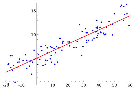
R^2 is the fraction of variance in y explained by the model, from 0 to 1. It is the most over-quoted statistic in applied work. A high R^2 does not mean the model is correct — one of Anscombe's four datasets from Chapter 7.7 is a curve fitted with a straight line and a respectable R^2. And R^2 always increases when you add a variable, even a random one, which is why adjusted R^2 exists and why comparing models on R^2 alone rewards overfitting.
Multiple regression uses several predictors:
y = \beta_0 + \beta_1x_1 + \beta_2x_2 + \cdots
Each coefficient is the effect of that variable holding the others constant, which is what makes regression a tool for separating tangled influences. It is also where the interpretation gets delicate: "holding constant" is a statement about the model, not about the world, and if two predictors always move together in reality, the model cannot separate them.
That is Chapter 4.2's multicollinearity. Nearly dependent columns make the coefficients wildly unstable — large, of unpredictable sign, and changing dramatically with a small change in the data — even while the predictions stay fine.
Assumptions worth checking: the relationship is linear, the errors are independent, their spread is constant across the range, and they are roughly normal. Plot the residuals against the fitted values; a pattern there means an assumption has failed.
Logistic regression handles a yes/no outcome by modelling the log odds (Chapter 7.2) rather than the value itself, and running it through the logistic curve of Chapter 6.1 to produce a probability. It is the workhorse of credit scoring, medical risk prediction and spam classification, and it is the simplest model in Volume I, 12.3.
6. Experimental design
The best statistics cannot rescue a bad study. Three ideas do most of the work.
Randomisation. Assign treatment at random. This is what lets you claim causation rather than correlation, because randomisation balances all other factors — including the ones you did not think of and cannot measure — between the groups on average. It is the single most important idea in experimental science.
Control groups. Without one you cannot separate the treatment from regression to the mean, natural recovery, or the placebo effect.
Blinding. Participants who know they got the treatment respond differently. Experimenters who know which group they are assessing score differently, usually without realising. Double-blind means neither knows.
A/B testing is randomised controlled trials applied to software, and the same rules apply: randomise properly, decide the sample size before starting, do not peek and stop early when the numbers look good, and correct for multiple comparisons if you are testing several metrics. Peeking is p-hacking with a friendly interface, and every experimentation platform has to defend against it.
Every formula above, built from scratch
None of the results in this chapter are worth memorising, because each one can be rebuilt in under a minute from something simpler. What follows is that rebuilding, one result at a time, so the formula and the reason for it sit on the same page as the explanation that needed them.
Hypothesis testing
\text{test statistic} = \frac{\text{estimate} - \text{value under } H_0}{\text{standard error}}
Every standard test is that one line with different pieces filled in.
| Situation | Statistic |
|---|---|
| Mean, \sigma known | z = \frac{\bar x - \mu_0}{\sigma/\sqrt n} |
| Mean, \sigma estimated | t = \frac{\bar x-\mu_0}{s/\sqrt n}, n-1 df |
| Proportion | z = \frac{\hat p - p_0}{\sqrt{p_0(1-p_0)/n}} |
| Two means | t = \frac{\bar x_1-\bar x_2}{\sqrt{s_1^2/n_1+s_2^2/n_2}} |
| Counts in categories | \chi^2 = \sum\frac{(O-E)^2}{E} |
p\text{-value} = P(\text{a result at least this extreme} \mid H_0 \text{ true})
What the p-value is not. It is not the probability that the null hypothesis is true. It is not the probability the result happened by chance. It answers only: if there were really no effect, how often would data look at least this striking? Everything else requires Bayes' theorem and a prior.
| H_0 true | H_0 false | |
|---|---|---|
| Reject | Type I error, rate \alpha | correct |
| Do not reject | correct | Type II error, rate \beta |
\text{power} = 1-\beta
The two errors trade against each other: demanding more evidence before declaring an effect (smaller \alpha) means missing more real effects (larger \beta). The only way to improve both at once is more data.
Regression
\hat y = b_0+b_1x, \qquad b_1 = \frac{\sum(x_i-\bar x)(y_i-\bar y)}{\sum(x_i-\bar x)^2} = r\frac{s_y}{s_x}, \qquad b_0 = \bar y - b_1\bar x
This is the least-squares solution derived in 4.1 — vectors §8, written in statistical notation. Two facts follow immediately from the formula for b_0: the fitted line always passes through the point (\bar x, \bar y), and the residuals always sum to zero.
r = \frac{\sum(x_i-\bar x)(y_i-\bar y)}{\sqrt{\sum(x_i-\bar x)^2\sum(y_i-\bar y)^2}}, \qquad -1\le r\le 1
R^2 = \frac{\text{variation explained}}{\text{total variation}} = 1 - \frac{\sum(y_i-\hat y_i)^2}{\sum(y_i-\bar y)^2}
R^2 = 0.8 means the line accounts for 80% of the up-and-down in y. It says nothing about whether x causes y, whether a straight line was the right shape, or whether the model will hold outside the range of the data. Those three questions are where almost all real statistical damage is done.
7. Where this shows up in your life
Every medical claim you read. Ask about sample size, control group, effect size and whether it replicated.
Every A/B test at work. And the temptation to stop it early.
Every "studies show" headline. Publication bias means the published claim is systematically stronger than the truth.
Every business dashboard with a trend line. Regression, and its assumptions.
Every credit score and insurance quote. Logistic regression on your attributes.
Every conversation about whether an intervention worked. Ask what the comparison group was. If there was not one, there is no conclusion to draw.
Part 7 is finished. We have chance, distributions, estimation and inference. The next Part steps away from continuous quantities to the mathematics of discrete structures — sets, logic, proof and graphs — which is the mathematics that computing is actually built from.
More places these turn up
Bayes' theorem is what makes a medical screening result meaningful or misleading, and it is worth doing the arithmetic before worrying about a positive test for a rare condition. The central limit theorem is why a poll of 1,000 people can describe a country of 60 million, and its \sqrt n is why the margin of error is about 3% rather than 0.3%. The Poisson distribution schedules staff at a call centre and stocks a shelf. Regression is behind every insurance premium you are quoted. And the p-value, misunderstood at scale, is a large part of why so many published findings fail to replicate — the story told in 7.8.
Next: 7.P — Worked Problems works through counting, Bayes with real numbers, distributions, a confidence interval and a full hypothesis test, step by step.