Appearance
3.4 — Coordinate Geometry: Where Algebra Meets Shape
The story is that René Descartes, lying ill in bed, watched a fly walking on the ceiling and realised he could describe its position at any moment with two numbers: its distance from one wall and its distance from the other. The story is probably invented. The idea is not, and it is one of the half-dozen genuinely revolutionary ideas in mathematics.
Before Descartes' La Géométrie (1637), geometry and algebra were separate subjects with separate methods. After it, every geometric shape is an equation and every equation is a shape. A problem that is hard in one language can be translated into the other and become easy. This fusion is called analytic geometry or coordinate geometry, and it made calculus possible thirty years later.

1. The coordinate plane
Draw two perpendicular number lines crossing at their zeros. The horizontal one is the x-axis, the vertical one the y-axis, and their crossing point is the origin. Any point in the plane is now named by an ordered pair (x, y): how far right, then how far up.
The order matters. (3, 5) and (5, 3) are different points. The convention is always horizontal first, and it is universal.
The axes cut the plane into four quadrants, numbered anticlockwise starting from the top right, where both coordinates are positive.
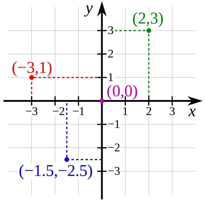
Screen coordinates run the other way
In every graphics system — your browser's canvas, a phone screen, an image file — the origin is at the top left and y increases downward. This is inherited from how cathode-ray televisions scanned an image, line by line from the top.
So a shape that looks right on paper appears upside down on screen unless you flip it. Volume I, 6.9 covers the graphics consequences. It is one of the most common sources of "why is my drawing mirrored" confusion, and the answer is always that the two conventions disagree about which way is up.
2. The two formulas everything is built on
Distance between two points. Draw the horizontal and vertical gaps between (x_1,y_1) and (x_2,y_2); they form a right triangle with the direct line as hypotenuse. Pythagoras from Chapter 3.2:
d = \sqrt{(x_2-x_1)^2 + (y_2-y_1)^2}
That is the entire content of the formula — it is Pythagoras with coordinates.
Midpoint. Average each coordinate separately:
M = \left(\frac{x_1+x_2}{2}, \frac{y_1+y_2}{2}\right)
Worked example. From (1,2) to (4,6): the gaps are 3 and 4, so the distance is \sqrt{9+16} = 5, and the midpoint is (2.5, 4).
These extend without modification to three dimensions, by adding a z term under the root, and to any number of dimensions — which is exactly what Chapter 4.1 does when a "point" becomes a list of 768 numbers.
3. Lines
Gradient, also called slope, measures steepness: the vertical change divided by the horizontal change, "rise over run".
m = \frac{y_2 - y_1}{x_2 - x_1}
Positive means uphill left to right, negative downhill, zero horizontal. A vertical line has an undefined gradient — the run is zero, and division by zero has no meaning (Chapter 1.2). That is not a flaw in the formula; it reflects a genuine fact that vertical lines are a special case in this framework.
The equation of a line. The most useful form is:
y = mx + c
where m is the gradient and c is the y-intercept, the height at which it crosses the vertical axis. Every non-vertical line has exactly one such equation.
Point-slope form is what you use when you know a point and a gradient:
y - y_1 = m(x - x_1)
Worked example. The line through (2,3) and (6,11). Gradient: m = \frac{11-3}{6-2} = 2. Then y - 3 = 2(x-2), so y = 2x - 1.
Parallel and perpendicular. Two lines are parallel when m_1 = m_2. They are perpendicular when
m_1 m_2 = -1
that is, when one gradient is the negative reciprocal of the other. A line of gradient \frac{2}{3} is perpendicular to one of gradient -\frac{3}{2}.
Why: rotating a line by 90° swaps the rise and the run and flips one sign, because what was horizontal displacement becomes vertical. Chapter 4.2 shows this cleanly as a matrix rotation.
4. Circles and conics as equations
A circle of radius r centred at (a,b) is the set of points at distance r from the centre. Write that with the distance formula and square both sides:
(x-a)^2 + (y-b)^2 = r^2
Centred at the origin it is x^2 + y^2 = r^2.
Sometimes a circle arrives expanded and disguised:
x^2 + y^2 - 6x + 4y - 12 = 0
Complete the square from Chapter 2.3 in x and in y separately:
(x^2 - 6x) + (y^2 + 4y) = 12
(x-3)^2 - 9 + (y+2)^2 - 4 = 12
(x-3)^2 + (y+2)^2 = 25
A circle of radius 5 centred at (3, -2). Completing the square is what turns an unreadable equation into a picture.
The conic sections of Chapter 3.3 all have equations of second degree, and the general form is:
Ax^2 + Bxy + Cy^2 + Dx + Ey + F = 0
Which curve you get is decided by the discriminant B^2 - 4AC — the same discriminant idea as Chapter 2.3. Negative gives an ellipse (or circle), zero gives a parabola, positive gives a hyperbola. In standard positions:
\text{Ellipse: } \frac{x^2}{a^2} + \frac{y^2}{b^2} = 1 \qquad \text{Hyperbola: } \frac{x^2}{a^2} - \frac{y^2}{b^2} = 1 \qquad \text{Parabola: } y = ax^2
One sign changes and the curve becomes a completely different shape. That is the kind of thing you can see in the algebra and would never guess from the geometry.
Proving the parabola's reflection property
Chapter 3.3 claimed that a parabola focuses parallel rays to a point. With coordinates this becomes checkable rather than mysterious.
Take y = \frac{x^2}{4p}, which has its focus at (0, p) and a horizontal directrix line at y = -p. The defining property is that every point on the curve is equidistant from the focus and the directrix.
A ray coming straight down hits the curve at (x_0, y_0). The distance it still has to travel to reach the focus equals the distance from that point down to the directrix, by the defining property. So every parallel ray, whatever its horizontal position, travels the same total distance to the focus — measuring from the directrix line. Equal distances means the waves arrive in step, which is exactly what "focusing" means for a signal.
That is why a satellite dish works, and why every ray arrives in phase rather than smeared. The algebraic definition made a physical fact obvious.
5. Transformations: moving a shape by changing its equation
If you know the graph of y = f(x), you can get many others by adjusting the equation. The rules are simple and the two directions behave oppositely, which is the part worth understanding rather than memorising.
| Change | Effect |
|---|---|
| f(x) + k | moves up by k |
| f(x + k) | moves left by k |
| a \cdot f(x) | stretches vertically by a |
| f(ax) | squashes horizontally by a |
| -f(x) | flips vertically |
| f(-x) | flips horizontally |
Why the horizontal ones are backwards. f(x+3) shifts left, not right, which feels wrong. Here is why: the new graph at x = -3 shows the value f(0), so whatever used to happen at 0 now happens at -3 — three units to the left. In general the input reaches its old value sooner, so the picture arrives earlier, so it moves left.
The rule that makes all six memorable: changes on the outside of f affect the output and behave as you expect; changes on the inside affect the input and do the opposite.
6. Where coordinates go next
Coordinates are not the only way to name a point, and choosing the right naming makes hard problems easy.
Polar coordinates give a distance and an angle, (r, \theta), instead of two distances. Conversion:
x = r\cos\theta, \qquad y = r\sin\theta, \qquad r = \sqrt{x^2+y^2}, \qquad \theta = \arctan\frac{y}{x}
A circle centred at the origin, which is x^2+y^2 = 25 in Cartesian, is simply r = 5 in polar. A spiral, which is horrible in Cartesian, is r = \theta. Anything with rotational symmetry is simpler in polar. This is also exactly the polar form of a complex number from Chapter 2.5 — the complex plane and the coordinate plane are the same plane with different arithmetic attached.
Three dimensions add a z-axis. A plane is ax + by + cz = d; a sphere is (x-a)^2+(y-b)^2+(z-c)^2 = r^2. Everything generalises, which is precisely why Chapter 4.1 can drop the pictures and work in any number of dimensions.
Latitude and longitude are a coordinate system on a sphere, and the reason a degree of longitude shrinks as you move away from the equator is that the coordinate grid is not uniform on a curved surface. That single fact is why every flat map distorts something, and why the Mercator projection makes Greenland look the size of Africa when it is fourteen times smaller.
Every formula above, built from scratch
None of the results in this chapter are worth memorising, because each one can be rebuilt in under a minute from something simpler. What follows is that rebuilding, one result at a time, so the formula and the reason for it sit on the same page as the explanation that needed them.
Coordinate geometry
d = \sqrt{(x_2-x_1)^2 + (y_2-y_1)^2}
Pythagoras, with the horizontal and vertical gaps as the two legs.
M = \left(\frac{x_1+x_2}{2}, \frac{y_1+y_2}{2}\right)
The midpoint is the average of the ends, coordinate by coordinate. More generally, the point dividing the segment in the ratio m:n is
\left(\frac{mx_2+nx_1}{m+n}, \frac{my_2+ny_1}{m+n}\right)
m = \frac{y_2-y_1}{x_2-x_1} = \frac{\text{rise}}{\text{run}}
Lines.
y = mx + c \quad\text{(gradient–intercept)}, \qquad y - y_1 = m(x-x_1) \quad\text{(point–gradient)}, \qquad ax+by+c=0 \quad\text{(general)}
Parallel lines have equal gradients. Perpendicular lines have gradients multiplying to -1.
Why the perpendicular rule is true. A line of gradient m goes 1 across and m up, so its direction is the vector (1, m). Rotating that by 90° gives (-m, 1) — rotating a vector a quarter turn swaps the coordinates and flips one sign, as 4.2 shows. The gradient of the new direction is \frac{1}{-m} = -\frac1m. And m \times \left(-\frac1m\right) = -1.
\text{Distance from } (x_0,y_0) \text{ to } ax+by+c=0: \quad d = \frac{|ax_0+by_0+c|}{\sqrt{a^2+b^2}}
Circle.
(x-h)^2 + (y-k)^2 = r^2
This is the distance formula with the distance fixed at r: every point exactly r from the centre (h,k). Expanding gives the general form x^2+y^2+Dx+Ey+F=0, and completing the square in x and in y turns any such equation back into centre-and-radius form.
The conic sections, in their standard positions:
| Curve | Equation | What it is |
|---|---|---|
| Parabola | y^2 = 4ax | points equidistant from a point and a line |
| Ellipse | \frac{x^2}{a^2}+\frac{y^2}{b^2}=1 | distances to two foci sum to a constant |
| Hyperbola | \frac{x^2}{a^2}-\frac{y^2}{b^2}=1 | distances to two foci differ by a constant |
For the ellipse, the foci sit at (\pm c, 0) with c^2 = a^2-b^2, and the constant sum is 2a. For the hyperbola, c^2 = a^2+b^2 and the asymptotes are y = \pm\frac ba x. The one sign change between the two equations is the whole difference between a planet's closed orbit and a comet's escape.
7. Where this shows up in your life
Every map application. A location is a coordinate pair; a route is a sequence of them; a "nearby" search is the distance formula run over a database.
Every screen and every image. A pixel is a coordinate, an image is a grid of them, and every drag, zoom and rotate is a transformation of Section 5 applied to coordinates. Volume I, 6.9 covers the canvas mathematics.
Every spreadsheet chart. Plotting is coordinate geometry, and a trendline is fitting an equation to points.
Every video game. Object positions, collision tests (is the distance between two centres less than the sum of the radii?), and camera transforms.
Every CNC machine, 3D printer and robot arm. They are told where to go in coordinates, and converting a desired hand position into joint angles is called inverse kinematics — coordinate geometry plus the trigonometry of the next chapter.
Every plot you have ever read, from a stock chart to a COVID case curve. It is Descartes' fly on the ceiling, and it is now so natural that seeing data any other way feels strange.
Coordinates handle position. What they do not yet handle is angle — we can say a line has gradient 2, but not what angle it makes, nor how to compute a side length from an angle. Trigonometry supplies that, and it turns out to describe not just triangles but every repeating thing in nature.