Appearance
8.5 — Recurrences and Growth
A pair of rabbits takes one month to mature, then produces a new pair every month thereafter, and rabbits never die. Starting with one newborn pair, how many pairs are there after a year?
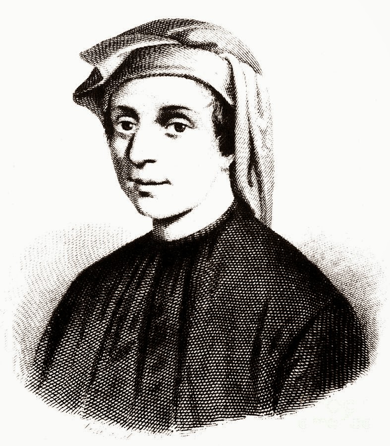
Leonardo of Pisa — known as Fibonacci — posed this in Liber Abaci in 1202, in the same book that introduced Hindu-Arabic numerals to Europe (Chapter 1.1). The answer is not a formula you can guess. It is a rule that defines each month from the previous ones:
F_n = F_{n-1} + F_{n-2}
Every pair alive last month is still alive, and every pair that was alive the month before is now old enough to breed. That is a recurrence relation, and this chapter is about solving them — because the running time of every recursive algorithm is one.
1. Solving a linear recurrence
F_n = F_{n-1}+F_{n-2}, \qquad F_0 = 0,\; F_1 = 1
giving 0,1,1,2,3,5,8,13,21,34,55,89,144,\ldots
The method: guess F_n = r^n and see what r must be. This is the same move as guessing e^{rt} for a differential equation in Chapter 6.2, and it works for the same reason — these are the functions that reproduce themselves under the operation involved.
r^n = r^{n-1}+r^{n-2}
Divide by r^{n-2}:
r^2 = r+1 \quad\Longrightarrow\quad r^2-r-1 = 0
The characteristic equation. By the quadratic formula:
r = \frac{1\pm\sqrt5}{2}
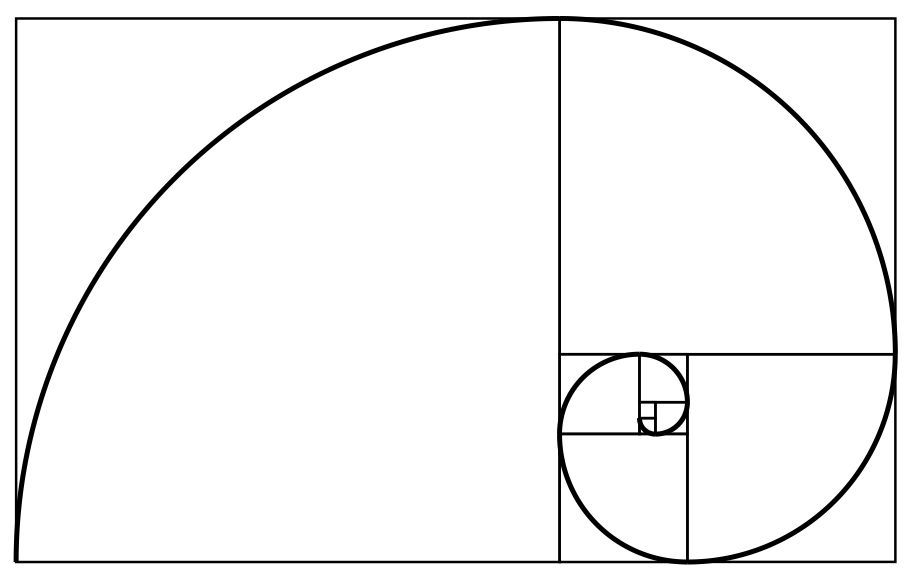
The positive root is \varphi \approx 1.618, the golden ratio of Chapter 1.7. The other is \psi = \frac{1-\sqrt5}{2}\approx-0.618.
Any combination A\varphi^n + B\psi^n satisfies the recurrence, and the initial values fix A and B:
F_n = \frac{\varphi^n-\psi^n}{\sqrt5}
Binet's formula. Chapter 4.5 reached the same result through eigenvalues, which is not a coincidence — the characteristic equation of the recurrence is the characteristic equation of the matrix.
Two things to notice.
A formula full of \sqrt5 always produces whole numbers. The irrational parts cancel exactly. Checking n=10: \frac{122.99 - (-0.0081)}{2.236} = 55. ✓
Since |\psi| \lt 1, its powers shrink to nothing, so for any decent n:
F_n \approx \frac{\varphi^n}{\sqrt5}, \text{ rounded to the nearest integer}
And that is why consecutive Fibonacci numbers approach the golden ratio — the dominant root takes over, exactly as the dominant eigenvalue did in Chapter 4.5.
2. The general method
For a linear recurrence with constant coefficients:
- Write the characteristic equation.
- Find its roots.
- Distinct roots: the solution is A_1r_1^n + A_2r_2^n+\cdots
- Repeated root r with multiplicity m: include r^n, nr^n, n^2r^n, \ldots up to n^{m-1}r^n. The extra factors of n are needed to get enough independent solutions, exactly as in Chapter 6.2.
- Complex roots: by Euler's formula they give oscillating solutions, so the sequence wobbles.
- Use the initial conditions to pin the constants.
The pattern to notice: recurrences and linear differential equations are the same theory. One steps in whole numbers, the other flows continuously, and both are solved by a characteristic equation. That is why Chapter 9.5's Z-transform (for sequences) looks so much like the Laplace transform (for functions) — they are the discrete and continuous versions of one idea.
3. Divide-and-conquer recurrences
The kind that appears in algorithm analysis. Merge sort splits an array in half, sorts each half, and merges in linear time:
T(n) = 2T(n/2)+n
The Master theorem solves the whole family
T(n) = aT(n/b)+f(n)
by comparing f(n) against n^{\log_b a}, which measures the work at the leaves of the recursion tree.
| Case | Result |
|---|---|
| f(n) grows slower than n^{\log_b a} | T(n) = \Theta(n^{\log_b a}) — leaves dominate |
| f(n) = \Theta(n^{\log_b a}) | T(n)=\Theta(n^{\log_b a}\log n) — every level costs the same |
| f(n) grows faster | T(n)=\Theta(f(n)) — the top level dominates |
Merge sort: a=2, b=2, so n^{\log_2 2} = n, and f(n) = n. Case 2, giving \Theta(n\log n).
Binary search: T(n) = T(n/2)+1, so a=1, b=2, n^{\log_2 1} = n^0 = 1, and f(n)=1. Case 2, giving \Theta(\log n).
Karatsuba multiplication: the schoolbook method for multiplying two n-digit numbers takes n^2 digit multiplications. Karatsuba's 1960 method splits each number in half and uses a trick to need only three half-size multiplications instead of four:
T(n) = 3T(n/2)+n
n^{\log_2 3} = n^{1.585} grows faster than n, so case 1 gives \Theta(n^{1.585}). Faster than n^2, and this was the first time anyone beat the schoolbook method — Kolmogorov had conjectured it was optimal, and a 23-year-old student disproved him within a week of hearing the conjecture.
Why this is the whole of algorithm analysis. Volume I, 4.1 uses this machinery throughout, and the reason a recursive algorithm's cost is a recurrence is that the algorithm's structure is a recurrence.
4. Generating functions
A technique that looks like a party trick and is a genuine tool. Encode a whole sequence as the coefficients of a power series:
G(x) = a_0 + a_1x + a_2x^2 + \cdots
The variable x means nothing on its own — it is a bookkeeping device that keeps the terms separated.
For the Fibonacci numbers, the recurrence turns into an algebraic equation:
G(x) = \frac{x}{1-x-x^2}
Then partial fractions from Chapter 2.2 split it into two geometric series, and reading off the coefficients gives Binet's formula again — this time without guessing anything.
Why bother. Manipulating one function is often easier than manipulating an infinite family of terms. It handles recurrences that resist the characteristic-equation method, it makes counting problems with complicated constraints tractable, and multiplying two generating functions corresponds to combining two sequences by convolution — which is Chapter 9.4's operation, appearing here in discrete form.
5. Counting with recurrences
Tower of Hanoi. Move n discs between pegs, never placing a larger on a smaller. To move n: move the top n-1 aside, move the largest, move the n-1 back.
H_n = 2H_{n-1}+1, \qquad H_1 = 1
Solving gives H_n = 2^n - 1. For 64 discs that is about 1.8\times10^{19} moves — at one per second, roughly 585 billion years. The legend attached to the puzzle says monks are moving 64 golden discs and the world ends when they finish, and the arithmetic says we are safe.
Climbing stairs. How many ways to climb n steps taking 1 or 2 at a time? The last move was either a 1 (from step n-1) or a 2 (from step n-2), so C_n = C_{n-1}+C_{n-2} — Fibonacci again, arriving from a completely unrelated problem.
Catalan numbers.
C_n = \frac{1}{n+1}\binom{2n}{n} = 1,1,2,5,14,42,132,\ldots
They count an astonishing variety of things: the ways to correctly match n pairs of brackets, the shapes of a binary tree with n nodes, the ways to triangulate a polygon, the paths on a grid that never cross the diagonal. When a counting problem produces 1, 2, 5, 14, 42, look for a Catalan structure — it usually means the objects have a recursive left-part/right-part decomposition.
6. Growth rates
Ordering the standard growth rates, from slowest to fastest:
1 \lt \log n \lt \sqrt n \lt n \lt n\log n \lt n^2 \lt n^3 \lt 2^n \lt n! \lt n^n
What each means practically, assuming a machine doing a billion operations per second:
| Growth | n=10^6 | Feel |
|---|---|---|
| \log n | 20 steps | instant |
| n | 1 million | milliseconds |
| n\log n | 20 million | fast |
| n^2 | 10^{12} | ~17 minutes |
| 2^n | beyond astronomical | never |
The gap between n\log n and n^2 is the difference between a sort that finishes and one that does not, which is why merge sort and quicksort replaced bubble sort everywhere.
Stirling's approximation gives the size of a factorial:
n! \approx \sqrt{2\pi n}\left(\frac ne\right)^n
Both \pi and e, in a formula about counting arrangements. It is how you evaluate 100! without multiplying a hundred numbers, and it is used constantly in statistical mechanics and information theory.
Every formula above, built from scratch
None of the results in this chapter are worth memorising, because each one can be rebuilt in under a minute from something simpler. What follows is that rebuilding, one result at a time, so the formula and the reason for it sit on the same page as the explanation that needed them.
Combinatorial identities
\binom nk = \binom{n}{n-k}, \qquad \binom nk = \binom{n-1}{k-1}+\binom{n-1}{k}
\sum_{k=0}^n\binom nk = 2^n
Proof in one line. Put a=b=1 into the binomial theorem: (1+1)^n = \sum\binom nk. Or count directly: the left side counts subsets by size, the right counts all subsets at once, and they must agree.
\sum_{k=0}^n(-1)^k\binom nk = 0 \quad (n\ge1)
Put a=1, b=-1 into the binomial theorem: (1-1)^n = 0. So every finite set has exactly as many even-sized subsets as odd-sized ones.
\sum_{k=0}^{n}\binom nk^2 = \binom{2n}{n}
Why. Choosing n items from 2n can be organised by how many come from the first half: if k come from the first n, then n-k come from the second, giving \binom nk\binom{n}{n-k} = \binom nk^2 ways. Sum over k.
Derangements — permutations leaving nothing in its original place:
D_n = n!\sum_{k=0}^n\frac{(-1)^k}{k!} \approx \frac{n!}{e}
Where it comes from. Inclusion–exclusion: start with all n! arrangements, subtract those fixing at least one item, add back those fixing at least two, and so on. The approximation says that in a large group where everyone draws a name from a hat, the probability that nobody draws their own is about \frac1e = 36.8\% — and it barely changes whether the group is 10 people or 10 million.
Catalan numbers.
C_n = \frac{1}{n+1}\binom{2n}{n}
They count balanced bracket strings, the ways to triangulate a polygon, the shapes of binary trees with n nodes, and about sixty other things: 1, 1, 2, 5, 14, 42, 132, \ldots
Recurrence relations
a_n = c_1a_{n-1}+c_2a_{n-2}
The method, and it is the same idea as second-order differential equations in 6.2 — second order and resonance. Guess a_n = r^n and substitute:
r^n = c_1r^{n-1}+c_2r^{n-2}
Divide by r^{n-2}:
r^2 = c_1r+c_2 \quad \Rightarrow \quad r^2-c_1r-c_2 = 0
That is the characteristic equation. Then:
- distinct roots r_1\ne r_2: a_n = Ar_1^n+Br_2^n
- repeated root r: a_n = (A+Bn)r^n
with A and B fixed by the starting values.
Binet's formula for Fibonacci, derived in full
F_n = F_{n-1}+F_{n-2}, \qquad F_0=0,\ F_1=1
Step 1 — the characteristic equation.
r^2 = r+1 \quad \Rightarrow \quad r^2-r-1=0
Step 2 — solve it.
r = \frac{1\pm\sqrt5}{2}
The positive root is the golden ratio \varphi = \frac{1+\sqrt5}{2} = 1.618034, and the other is \psi = \frac{1-\sqrt5}{2} = -0.618034.
Step 3 — write the general solution.
F_n = A\varphi^n + B\psi^n
Step 4 — use the starting values. From F_0 = 0:
A+B = 0 \quad \Rightarrow \quad B = -A
From F_1 = 1:
A\varphi + B\psi = 1 \quad \Rightarrow \quad A(\varphi-\psi) = 1
And \varphi - \psi = \frac{1+\sqrt5}{2}-\frac{1-\sqrt5}{2} = \sqrt5, so A = \frac{1}{\sqrt5}.
Step 5 — the formula.
F_n = \frac{\varphi^n-\psi^n}{\sqrt5} = \frac{1}{\sqrt5}\left[\left(\frac{1+\sqrt5}{2}\right)^n - \left(\frac{1-\sqrt5}{2}\right)^n\right]
Check at n=5. \varphi^5 = 11.0902 and \psi^5 = -0.0902, so F_5 = \frac{11.0902+0.0902}{\sqrt5} = \frac{11.1803}{2.2361} = 5 ✓
The startling part. An expression stuffed with \sqrt5 produces a whole number every single time, because the irrational parts cancel exactly. And since |\psi| < 1, the second term shrinks towards zero, so for any n\ge1:
F_n = \text{the nearest whole number to } \frac{\varphi^n}{\sqrt5}
Consecutive Fibonacci numbers therefore have a ratio approaching \varphi, which is why the golden ratio appears in sunflower seed spirals, pine cones and the branching of plants — all of which grow by adding the last two stages.
The Master theorem, for divide-and-conquer
T(n) = aT\!\left(\frac nb\right)+f(n)
Compare f(n) with n^{\log_b a}:
| Case | Result |
|---|---|
| f(n) grows slower | T(n) = \Theta(n^{\log_b a}) |
| f(n) = \Theta(n^{\log_b a}) | T(n) = \Theta(n^{\log_b a}\log n) |
| f(n) grows faster | T(n)=\Theta(f(n)) |
What the comparison means. a is how many pieces you recurse on, b is how much smaller each is, and f(n) is the work of splitting and recombining. The exponent \log_b a measures the total work at the bottom of the recursion. The three cases are: the leaves dominate, everything is balanced, or the top level dominates.
Merge sort has a=2, b=2, f(n)=n. Then n^{\log_2 2} = n, which matches f(n) — case two, giving \Theta(n\log n).
Binary search has a=1, b=2, f(n)=1. Then n^{\log_2 1} = n^0 = 1, matching f — case two again, giving \Theta(\log n).
7. Where this shows up in your life
Every recursive algorithm's running time. A recurrence, solved by the Master theorem.
Every compound growth process. Population, interest, viral spread — first-order recurrences.
Every dynamic programming solution. Volume I, 4.10 is entirely about recognising a recurrence and computing it without recomputing subproblems.
Every performance conversation. "It is O(n^2)" means the table in Section 6, and knowing that table is what lets you say whether a proposed approach will survive contact with production data.
Every sunflower and pine cone. Fibonacci spirals, which arise because that packing leaves the fewest gaps.
Every bracket-matching parser and every binary tree count. Catalan numbers.
One structure appears in almost every applied problem and deserves its own chapter: things connected to other things. That is a graph, and it is the most useful object in discrete mathematics.