Appearance
2.2 — Polynomials
Drop a stone from a cliff. Its height above the ground after t seconds is
h(t) = 45 - 4.9t^2
Design an arch, model a company's profit against price, fit a curve through data points, compute a sine on a processor that has no sine circuit — in every one of these you end up with an expression that is a sum of powers of a variable, each multiplied by a number. That is a polynomial, and it is the most-used family of functions in applied mathematics for a simple reason: a computer can evaluate one using nothing but addition and multiplication.
1. The definition and the vocabulary
A polynomial in x is a sum of terms, each a number times a whole-number power of x:
p(x) = a_n x^n + a_{n-1}x^{n-1} + \cdots + a_1 x + a_0
The numbers a_n, \ldots, a_0 are the coefficients. The largest power with a nonzero coefficient is the degree, and a_n is the leading coefficient. The lonely a_0 with no x is the constant term.
What is not allowed is what makes polynomials well-behaved: no negative powers (x^{-1} is out), no fractional powers (\sqrt{x} = x^{1/2} is out), no variable in a denominator or an exponent. Only whole-number powers, only finitely many terms.
The degrees have names you will hear constantly:
| Degree | Name | Example | Shape of graph |
|---|---|---|---|
| 0 | constant | 7 | horizontal line |
| 1 | linear | 3x - 2 | straight line |
| 2 | quadratic | x^2 - 5x + 6 | parabola |
| 3 | cubic | x^3 - x | one or two bends |
| 4 | quartic | x^4 + 1 | up to three bends |
"Quadratic" comes from Latin quadratus, square — degree two is the squaring degree, exactly as in Chapter 1.4.
A useful mental rule: a polynomial of degree n has at most n-1 turning points and at most n roots. So a cubic can wiggle at most twice, and a quadratic exactly once. Knowing the degree tells you the shape before you plot anything.
2. Arithmetic on polynomials
Adding means collecting like terms — terms with the same power. You can only add x^2 to x^2, for the same reason from Chapter 1.3 that you can only add quarters to quarters.
(3x^2 + 2x - 1) + (x^2 - 5x + 4) = 4x^2 - 3x + 3
Multiplying means everything meets everything, from Chapter 2.1.
(x + 2)(x^2 - 3x + 1) = x^3 - 3x^2 + x + 2x^2 - 6x + 2 = x^3 - x^2 - 5x + 2
Notice the degrees add: degree 1 times degree 2 gives degree 3. That is always true, and it is a small but genuinely useful check on your arithmetic.
Dividing works like long division of numbers, and looks intimidating only because the layout is unfamiliar. Divide x^3 - 2x^2 - 4 by x - 3:
Ask what times x gives x^3. Answer x^2. Multiply x^2(x-3) = x^3 - 3x^2 and subtract, leaving x^2 - 4. Ask what times x gives x^2. Answer x. Multiply x(x-3) = x^2 - 3x and subtract, leaving 3x - 4. Ask what times x gives 3x. Answer 3. Multiply 3(x-3) = 3x - 9 and subtract, leaving 5.
\frac{x^3 - 2x^2 - 4}{x - 3} = x^2 + x + 3 \;+\; \frac{5}{x-3}
Quotient x^2 + x + 3, remainder 5 — exactly the structure of \frac{17}{5} = 3 + \frac{2}{5}. Polynomials behave like integers in this respect, and Chapter 8.4 explains that this is not a coincidence but a shared algebraic structure.
3. Roots, factors, and the theorem that links them
A root (or zero) of p(x) is a value of x making p(x) = 0. On a graph, it is where the curve crosses the horizontal axis.
The Remainder Theorem. When you divide p(x) by (x - c), the remainder is exactly p(c).
Check with the division above: p(x) = x^3 - 2x^2 - 4 divided by x - 3 left remainder 5. And p(3) = 27 - 18 - 4 = 5. It works, and the reason is one line. Write p(x) = (x-c)q(x) + r. Substitute x = c: the first term vanishes, leaving p(c) = r.
The Factor Theorem is the immediate consequence: (x - c) is a factor of p(x) exactly when p(c) = 0.
This is the practical tool. To factor a cubic, hunt for a root by trying small numbers; when one works, you have a factor, and dividing by it leaves a quadratic you can handle.
Worked example. Factor x^3 - 6x^2 + 11x - 6.
Try x=1: 1 - 6 + 11 - 6 = 0. A root. So (x-1) is a factor. Divide:
x^3 - 6x^2 + 11x - 6 = (x-1)(x^2 - 5x + 6)
The quadratic factors by inspection — which two numbers multiply to 6 and add to -5? Minus two and minus three:
= (x-1)(x-2)(x-3)
Roots at 1, 2 and 3.
Where to look for roots. The rational root theorem narrows the search enormously: any rational root \frac{p}{q} in lowest terms must have p dividing the constant term and q dividing the leading coefficient. For x^3 - 6x^2 + 11x - 6, the leading coefficient is 1, so q = 1, and p divides 6. The only candidates are \pm1, \pm2, \pm3, \pm6 — eight numbers to try instead of infinitely many.
4. How many roots does a polynomial have?
The Fundamental Theorem of Algebra: every polynomial of degree n with complex coefficients has exactly n roots among the complex numbers, counting repeats.
Two things need unpacking there.
"Counting repeats" handles cases like (x-2)^2 = x^2 - 4x + 4, which has degree 2 and only one visible root at x=2. We say 2 is a root of multiplicity 2, and the count comes out right. Graphically, a root of even multiplicity touches the axis and turns back; a root of odd multiplicity crosses it.
"Among the complex numbers" is the catch. Over the reals the theorem is false: x^2 + 1 = 0 has no real solution, since no real number squares to -1. It has two complex ones, and Chapter 2.5 builds them.
So the honest statement over the reals is: a degree-n polynomial has at most n real roots, and the missing ones come in complex pairs. Chapter 2.5 explains why they must pair up.
Gauss gave the first broadly accepted proof in his 1799 doctoral thesis, at the age of 22, and returned to it three more times across his life to give better proofs. Despite the name, it is not really a theorem of algebra — every known proof needs some analysis or topology — but the name stuck.
5. What the graph looks like, without plotting points
You can sketch any polynomial from four observations, which is much faster than making a table of values.
End behaviour, from the leading term. For very large |x|, the highest power dwarfs everything else. So:
- Even degree, positive leading coefficient: both ends go up.
- Even degree, negative: both ends go down.
- Odd degree, positive: down on the left, up on the right.
- Odd degree, negative: the reverse.
Roots, from the factors. Each factor (x-c) puts a crossing at c.
Behaviour at each root, from its multiplicity. Odd multiplicity crosses; even multiplicity touches and bounces.
The y-intercept, from the constant term. At x=0 everything with an x vanishes, so the curve passes through (0, a_0).
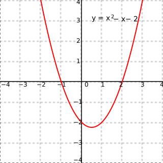
Worked sketch. p(x) = (x+2)(x-1)^2.
Degree 3, positive leading coefficient, so it comes up from the bottom left and exits top right. It crosses at x=-2. At x=1 the factor is squared, so it touches the axis and turns back without crossing. At x=0, p(0) = 2 \times 1 = 2. That is enough to draw the curve, and the drawing is right.
6. Evaluating efficiently: Horner's method
To compute p(x) = 2x^3 - 6x^2 + 2x - 1 at x = 3 the obvious way, you calculate x^3, x^2, multiply each by its coefficient, and add. That is six multiplications and three additions, and it gets worse fast for higher degrees.
Rewrite by repeatedly factoring out x:
p(x) = ((2x - 6)x + 2)x - 1
Now evaluate from the inside out at x=3: 2(3) - 6 = 0; 0 \times 3 + 2 = 2; 2 \times 3 - 1 = 5. Three multiplications instead of six, and for degree n it is n multiplications instead of about 2n.
js
// Horner's method. coeffs are highest power first.
function horner(coeffs, x) {
  let result = coeffs[0];                    // (1)
  for (let i = 1; i < coeffs.length; i++) {
    result = result * x + coeffs[i];         // (2)
  }
  return result;
}
horner([2, -6, 2, -1], 3);                   // → 5
Line (1) starts with the leading coefficient. Line (2) is the entire algorithm: multiply what you have so far by x, then add the next coefficient down. Each pass through the loop consumes one coefficient and does one multiply and one add.
This is not a curiosity. It is what runs inside your processor when you call Math.sin or exp — those functions are computed from polynomial approximations (Chapter 5.8 explains where the approximations come from), evaluated by Horner or a close relative, millions of times a second. The method was published by William Horner in 1819 and was known to Chinese mathematicians by the thirteenth century.
7. Fitting a polynomial through points
Given n+1 points with distinct x values, there is exactly one polynomial of degree at most n passing through all of them.
Two points determine a line. Three points determine a parabola. This is the mathematical basis of curve fitting, and it has a warning attached.
Interpolation is safe; extrapolation is not. A polynomial forced through your data points will do whatever it likes between and beyond them, and high-degree fits oscillate wildly near the edges — a phenomenon named Runge's phenomenon after Carl Runge, who found it in 1901. Fitting a degree-12 polynomial through 13 data points gives you a curve that hits every point and is useless for prediction.
The practical response is to fit a low-degree polynomial that passes near the points rather than through them — the least squares fit of Chapter 7.8 — or to use many low-degree pieces joined smoothly, called splines, which is how every font on your screen and every curve in a drawing program is defined.
8. Partial fractions, and why they matter later
A rational function is one polynomial divided by another. Often it can be split into a sum of simpler pieces:
\frac{5x - 4}{x^2 - x - 2} = \frac{5x-4}{(x-2)(x+1)} = \frac{A}{x-2} + \frac{B}{x+1}
To find A and B, multiply through by the denominator:
5x - 4 = A(x+1) + B(x-2)
This must hold for every x, so pick convenient values. At x = 2: 6 = 3A, so A = 2. At x = -1: -9 = -3B, so B = 3. Therefore:
\frac{5x-4}{x^2-x-2} = \frac{2}{x-2} + \frac{3}{x+1}
Verify by combining them back over a common denominator; you get the original.
Why bother. Because integrating \frac{1}{x-2} is easy and integrating the original is not (Chapter 5.6), and because inverting a Laplace transform is done by exactly this splitting (Chapter 9.5), which is how every electrical circuit and control system in Volume III gets solved. Partial fractions look like pointless algebra until the moment you need them, at which point they are the whole technique.
Every formula above, built from scratch
None of the results in this chapter are worth memorising, because each one can be rebuilt in under a minute from something simpler. What follows is that rebuilding, one result at a time, so the formula and the reason for it sit on the same page as the explanation that needed them.
The cubes
The cube of a sum
(a+b)^3 = a^3 + 3a^2b + 3ab^2 + b^3
Where it comes from. Take what you already have and multiply once more:
(a+b)^3 = (a+b)^2(a+b) = (a^2 + 2ab + b^2)(a+b)
Multiply out term by term:
= a^3 + a^2b + 2a^2b + 2ab^2 + ab^2 + b^3
Collect the like terms — a^2b + 2a^2b = 3a^2b, and 2ab^2 + ab^2 = 3ab^2:
= a^3 + 3a^2b + 3ab^2 + b^3
The coefficients 1, 3, 3, 1 are the fourth row of Pascal's triangle, and §6 explains why they must be.
(a-b)^3 = a^3 - 3a^2b + 3ab^2 - b^3
The signs alternate because each b carries a minus with it, so terms with an odd number of b's come out negative.
The sum of two cubes — the one people never see derived
a^3 + b^3 = (a+b)(a^2 - ab + b^2)
Read it aloud. "a cubed plus b cubed equals a plus b, times a squared minus a-b plus b squared."
Verify first, then understand. Multiply the right side out. Take each term of (a+b) across the second bracket:
a(a^2 - ab + b^2) = a^3 - a^2b + ab^2
b(a^2 - ab + b^2) = a^2b - ab^2 + b^3
Add the two lines. Line one has -a^2b and line two has +a^2b, so they cancel. Line one has +ab^2 and line two has -ab^2, so those cancel too. All that survives is:
a^3 + b^3
Where the factor (a+b) comes from in the first place, so you could have found this yourself. Think of a^3 + b^3 as a polynomial in a, with b held fixed. Put a = -b into it:
(-b)^3 + b^3 = -b^3 + b^3 = 0
The expression is zero when a = -b. The factor theorem — proved in 2.2 — says that if a polynomial vanishes at a = -b, then (a+b) is a factor of it. So (a+b) must divide a^3+b^3, and the other factor is whatever you get from the division. Divide and you get a^2 - ab + b^2. Nothing was guessed.
The difference of cubes, by the same route. Put a = b into a^3 - b^3 and you get zero, so (a - b) is a factor:
a^3 - b^3 = (a-b)(a^2 + ab + b^2)
The memory hook that is actually a reason. In both, the quadratic factor is a^2 \pm ab + b^2, and the sign in the middle is the opposite of the sign in the linear factor. That is not decoration: it is what makes the cross terms cancel, exactly as it was in §2.
The general pattern behind all of it.
a^n - b^n = (a-b)\left(a^{n-1} + a^{n-2}b + a^{n-3}b^2 + \cdots + b^{n-1}\right)
Every a^n - b^n has a - b as a factor, for every n. This is the identity behind the geometric series of §7, and it is why 2^{11} - 1 is not prime but 2^{13}-1 might be — a thread picked up in 1.5.
Two more that turn up constantly
(a+b+c)^2 = a^2+b^2+c^2+2ab+2bc+2ca
Every letter squared once, plus twice every pair, because each pair can be chosen in two orders.
a^3+b^3+c^3-3abc = (a+b+c)(a^2+b^2+c^2-ab-bc-ca)
A useful consequence: when a+b+c=0, the whole left side collapses and a^3+b^3+c^3 = 3abc.
The binomial theorem
(a+b)^n = \sum_{k=0}^{n}\binom{n}{k}a^{n-k}b^{k}, \qquad \binom{n}{k} = \frac{n!}{k!\,(n-k)!}
Read it aloud. "a plus b to the n equals the sum, for k from zero to n, of n-choose-k times a to the n minus k times b to the k."
Where it comes from — by counting, not by algebra. Write (a+b)^n as n brackets side by side:
\underbrace{(a+b)(a+b)\cdots(a+b)}_{n \text{ brackets}}
Multiplying out means: go along the brackets, take either the a or the b from each, multiply your choices, and do this for every possible set of choices. Any run in which you took b from exactly k brackets contributes a^{n-k}b^k. So the question "what is the coefficient of a^{n-k}b^k?" is really the question "in how many ways can I choose which k of the n brackets hand me a b?" — and that count is \binom{n}{k}, derived in 7.1.
That is the whole proof. The binomial coefficients are not a mysterious pattern; they are the number of ways to pick k things from n.
Pascal's triangle and the rule behind it.
\binom{n}{k} = \binom{n-1}{k-1} + \binom{n-1}{k}
Each entry is the sum of the two above it. Why: to choose k items from n, look at the last item. Either you take it — and then you need k-1 more from the remaining n-1 — or you leave it, and need all k from the remaining n-1. Every selection falls into exactly one of those two cases, so the counts add.
A worked expansion. (2x - 3)^4. Here a = 2x, b = -3, n = 4, and the coefficients from row four are 1, 4, 6, 4, 1:
(2x)^4 + 4(2x)^3(-3) + 6(2x)^2(-3)^2 + 4(2x)(-3)^3 + (-3)^4
= 16x^4 - 96x^3 + 216x^2 - 216x + 81
Note (-3)^2 = +9 while (-3)^3 = -27: the signs alternate on their own, so there is no separate sign rule to remember.
Sequences and series
Arithmetic: a constant difference
a_n = a_1 + (n-1)d, \qquad S_n = \frac{n}{2}\left(a_1 + a_n\right) = \frac{n}{2}\left(2a_1 + (n-1)d\right)
Where the n-th term comes from. Starting at a_1, you add d once to reach the second term, twice to reach the third — so n-1 times to reach the n-th.
Where the sum comes from — Gauss's trick. Write the sum forwards, then write it again backwards underneath:
\begin{aligned} S_n &= a_1 + (a_1+d) + (a_1+2d) + \cdots + a_n \\ S_n &= a_n + (a_n-d) + (a_n-2d) + \cdots + a_1 \end{aligned}
Add the two lines column by column. In every column, whatever is added to the top is subtracted from the bottom, so every column totals the same thing: a_1 + a_n. There are n columns, so
2S_n = n(a_1+a_n) \quad \Rightarrow \quad S_n = \frac{n}{2}(a_1+a_n)
The story of the schoolboy Gauss summing 1 to 100 in seconds is in 11.2; the pairing is exactly this. For 1+2+\cdots+n:
S_n = \frac{n(n+1)}{2}
Geometric: a constant ratio
a_n = a_1 r^{\,n-1}, \qquad S_n = a_1\frac{1-r^n}{1-r} \;(r \ne 1), \qquad S_\infty = \frac{a_1}{1-r} \;\text{ if } |r|<1
Where the finite sum comes from — the subtraction trick. Write the sum, multiply the whole thing by r, and subtract:
S_n = a_1 + a_1r + a_1r^2 + \cdots + a_1r^{n-1}
rS_n = \qquad\; a_1r + a_1r^2 + \cdots + a_1r^{n-1} + a_1r^{n}
Subtract the second line from the first. Every term in the middle appears in both lines and cancels; only the very first term of the top line and the very last of the bottom survive:
S_n - rS_n = a_1 - a_1r^n
S_n(1-r) = a_1(1-r^n) \quad \Rightarrow \quad S_n = a_1\frac{1-r^n}{1-r}
Where the infinite sum comes from. If |r| < 1, then r^n shrinks towards zero as n grows — half of a half of a half eventually rounds to nothing. Put r^n \to 0 into the finite formula:
S_\infty = \frac{a_1}{1-r}
If |r| \ge 1 the terms do not shrink, the sum grows without limit, and the formula is meaningless. This condition is not a technicality; it is the whole difference between a convergent and a divergent series, treated properly in 5.8.
A worked case. 0.9 + 0.09 + 0.009 + \cdots has a_1 = 0.9 and r = 0.1:
S_\infty = \frac{0.9}{1-0.1} = \frac{0.9}{0.9} = 1
which is the same 0.\overline{9} = 1 that appeared in 1.3 — fractions decimals ratios, now proved a second way.
The power sums
\sum_{k=1}^{n} k = \frac{n(n+1)}{2}, \qquad \sum_{k=1}^{n} k^2 = \frac{n(n+1)(2n+1)}{6}, \qquad \sum_{k=1}^{n} k^3 = \left(\frac{n(n+1)}{2}\right)^2
The third is startling: the sum of the first n cubes is the square of the sum of the first n numbers. 1+8+27 = 36 = 6^2 = (1+2+3)^2. All three are proved by induction in 8.3.
Algebraic fractions and partial fractions
\frac{P(x)}{(x-p)(x-q)} = \frac{A}{x-p} + \frac{B}{x-q}
Why anybody wants this. Going the other way — adding two simple fractions — is easy. Going backwards, splitting a complicated fraction into simple ones, is what makes integration possible in 5.6 and what makes the Laplace transform usable in 9.5. It is worth the effort because the pieces are things you can handle and the whole is not.
The method, worked. Split \dfrac{5x-7}{(x-1)(x-3)}.
Write the target form and clear the denominators by multiplying both sides by (x-1)(x-3):
5x - 7 = A(x-3) + B(x-1)
This must hold for every x, so choose values of x that kill one unknown at a time. That freedom is the trick.
Put x = 1: the B term dies because (1-1) = 0.
5(1) - 7 = A(1-3) \quad \Rightarrow \quad -2 = -2A \quad \Rightarrow \quad A = 1
Put x = 3: now the A term dies.
5(3) - 7 = B(3-1) \quad \Rightarrow \quad 8 = 2B \quad \Rightarrow \quad B = 4
\frac{5x-7}{(x-1)(x-3)} = \frac{1}{x-1} + \frac{4}{x-3}
Check by adding them back: \frac{(x-3) + 4(x-1)}{(x-1)(x-3)} = \frac{5x-7}{(x-1)(x-3)} ✓
The two variations you will meet. A repeated factor (x-p)^2 needs both \frac{A}{x-p} and \frac{B}{(x-p)^2}. An irreducible quadratic x^2+px+q (one with no real roots) needs a linear top: \frac{Ax+B}{x^2+px+q}.
9. Where this shows up in your life
Every projectile. Height under gravity is a quadratic in time, which is why a thrown ball traces a parabola and why Chapter 2.3 spends a whole page on quadratics.
Every trend line in a spreadsheet. Excel's polynomial trendline is Section 7, complete with the extrapolation danger.
Every curve in every font and vector drawing. Letters are built from cubic Bézier curves — cubic polynomials with control points. Volume I, 6.9 covers the graphics side.
Every Math.sin, Math.exp and Math.log call. Polynomial approximation plus Horner evaluation.
Every error-correcting code on a disk, a QR code, or a deep-space transmission. Reed–Solomon coding treats data as the coefficients of a polynomial and recovers lost values by reconstructing it from surviving points — the same "n+1 points determine a degree-n polynomial" fact as Section 7. Volume I, 1.8 covers error correction.
Degree one is solved by rearranging. Degree two has a complete formula that has been known for a thousand years and is worth deriving rather than memorising. That is the next chapter.