Appearance
9.3 — The Fourier Transform
A Fourier series needs a periodic function. A spoken word, a hand clap, a single heartbeat — these happen once and never repeat.
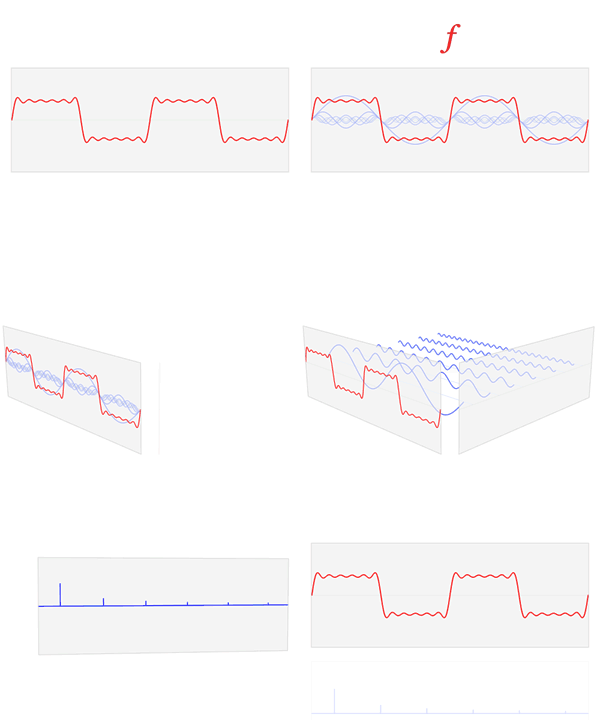
The extension is a limiting argument. Take a non-periodic signal and pretend it repeats with period T. Its Fourier series has harmonics spaced \frac{2\pi}{T} apart. Now let T grow. The harmonics crowd closer together, and in the limit they merge into a continuum.
The sum becomes an integral, and the discrete list of harmonic amplitudes becomes a continuous function of frequency.
\hat f(\omega) = \int_{-\infty}^{\infty}f(t)e^{-i\omega t}\,dt
f(t) = \frac{1}{2\pi}\int_{-\infty}^{\infty}\hat f(\omega)e^{i\omega t}\,d\omega
The first turns a signal into its spectrum; the second turns it back. Nothing is lost — the two descriptions carry identical information, just organised differently.
1. Reading the formula
\hat f(\omega) = \int f(t)e^{-i\omega t}dt
Multiply the signal by a pure tone of frequency \omega and add up the result. That is Chapter 9.1's detector, exactly. If the signal contains that frequency, the product is systematically in step and the integral is large. If not, the product oscillates and cancels to nearly nothing.
\hat f(\omega) is complex, and both parts mean something (Chapter 2.5):
- |\hat f(\omega)| is the amplitude at that frequency — how much of it is present.
- \arg\hat f(\omega) is the phase — where in its cycle that component sits.
Amplitude gets nearly all the attention and phase carries more of the structure than people expect. Take two photographs, swap their phase spectra while keeping their amplitudes, and each reconstructed image looks like the picture whose phase it borrowed. Amplitude says what frequencies are present; phase says where they line up, and lining up is what makes an edge.
2. The properties that make it useful
Linearity. The transform of a sum is the sum of the transforms. Straightforward and constantly relied upon.
Time shift becomes phase shift. Delaying a signal multiplies its transform by e^{-i\omega t_0} — the amplitudes are untouched and only the phases rotate. Delay does not change what frequencies are present, which is obviously true and pleasant to see fall out.
Differentiation becomes multiplication by i\omega.
\widehat{f'}(\omega) = i\omega\,\hat f(\omega)
This is the property that makes the transform a tool rather than a curiosity. A differential equation in time becomes an algebraic equation in frequency. Chapter 9.5 builds the engineering method on it.
Convolution becomes multiplication. Chapter 9.4 is about this one.
Scaling is reciprocal. Squeeze a signal in time and its spectrum spreads in frequency. A brief click contains all frequencies; a long steady tone contains almost one. Short in time means wide in frequency, always.
That reciprocity has a formal name and a famous consequence.
The uncertainty principle is a fact about waves
\Delta t \cdot \Delta\omega \ge \frac12
A signal cannot be sharply localised in both time and frequency. This is a theorem about Fourier transforms, provable in a page, with no physics in it at all.
The physics arrives when you add one experimental fact. Quantum mechanics says a particle's momentum is proportional to the spatial frequency of its wave, p = \hbar k. Substitute that into the mathematical inequality and you get
\Delta x\,\Delta p \ge \frac{\hbar}{2}
Heisenberg's uncertainty principle. It is not about measurement disturbing the system, and not about the limits of instruments. A particle described by a wave simply cannot have both a definite position and a definite momentum, for the same reason a sound cannot be both an instant and a pure tone. Volume IV, Chapter 7 develops the physics; the mathematics is entirely this chapter.
The same trade-off appears in music: to identify a pitch precisely you must listen for a while, which is why very short bass notes sound indistinct and why a spectrogram must choose between time detail and frequency detail.
3. The discrete version, and the algorithm that changed computing
A computer has samples, not a continuous function. The Discrete Fourier Transform is the finite version:
X_k = \sum_{n=0}^{N-1}x_ne^{-2\pi ikn/N}
N samples in, N complex numbers out.
Computed directly this costs N^2 operations — each of N outputs needs a sum over N inputs. For a one-second audio clip at 44,100 samples that is about two billion operations, and it was genuinely prohibitive.
In 1965 Cooley and Tukey published the Fast Fourier Transform, which does it in N\log N.
The idea is divide and conquer. Split the samples into even-indexed and odd-indexed halves, transform each half, and combine. The combination works because e^{-2\pi ik/N} raised to various powers takes only N distinct values — the roots of unity from Chapter 2.5 — and the two halves share them. That gives
T(N) = 2T(N/2)+N
which Chapter 8.5's Master theorem solves as \Theta(N\log N).
| N | N^2 | N\log_2 N | Speed-up |
|---|---|---|---|
| 1,024 | ~1 million | ~10,000 | 100× |
| 1 million | 10^{12} | 20 million | 50,000× |
That speed-up is not an optimisation, it is the difference between possible and impossible. Real-time audio processing, digital radio, medical imaging, JPEG and MP3 all exist because of it. It is routinely listed among the most important algorithms of the twentieth century.
And Gauss had it in 1805, in an unpublished notebook, while interpolating asteroid orbits — before Fourier published the series. It sat unnoticed in his collected works, in Latin, for 160 years.
4. Sampling: how a continuous signal becomes numbers
To digitise a signal you measure it at regular intervals. How often is often enough?
The Nyquist–Shannon sampling theorem: to reconstruct a signal exactly, sample at more than twice its highest frequency.
Human hearing reaches about 20 kHz, so audio CDs sample at 44.1 kHz — just over twice, with margin for the anti-aliasing filter. That is where the odd-looking 44,100 comes from, not from anything arbitrary.
What happens if you sample too slowly is aliasing: a high frequency masquerades as a lower one, because too few samples were taken to distinguish them.
You have seen it. Wagon wheels that appear to spin backwards in films — the wheel rotates nearly a full spoke-spacing between frames, so it appears to have moved slightly backwards. Film samples at 24 frames per second, far too slow for a spinning wheel. The same effect makes helicopter rotors look stationary on video.
In images it produces moiré patterns — the strange shimmering on a striped shirt in a photograph, where the fabric's stripe frequency exceeds what the sensor can resolve.
The fix is an anti-aliasing filter: remove frequencies above half the sampling rate before sampling. Once aliased, the damage cannot be undone, because the information needed to tell the two frequencies apart was never captured.
In computer graphics the same word means the same thing. A jagged diagonal line is aliasing — the pixel grid samples too coarsely for the edge's sharpness. Antialiasing filters before sampling, which is why the edge is drawn with intermediate shades.
5. Where the transform actually runs
Audio compression. MP3 and AAC transform to the frequency domain, then discard what you cannot hear. Psychoacoustic masking means a loud tone hides quieter ones nearby in frequency, so those can be thrown away entirely. Compression of 10:1 with little audible loss.
Image compression. JPEG splits an image into 8×8 blocks and applies a discrete cosine transform to each — a close relative of the Fourier transform using only cosines, chosen because it concentrates energy better for real images. High-frequency coefficients get quantised aggressively, since the eye is less sensitive to fine detail than to broad shading. The 8×8 block size is a compromise: larger blocks compress better and make the blocking artefacts more visible when they appear.
Noise cancellation. Sample the ambient sound, transform, and generate the inverse. The headphone produces a wave that cancels the noise, which works because the wave equation of Chapter 6.4 is linear and waves add.
Medical imaging. MRI does not measure the image directly — it measures the Fourier transform of the image, one frequency at a time, and reconstructs by inverting. The scanner's characteristic knocking noise is the gradient coils switching to select each frequency. CT reconstruction uses a related transform.
Radio and mobile networks. OFDM, the modulation behind Wi-Fi, 4G and 5G, splits data across many orthogonal subcarriers, and both the transmitter and receiver are running FFTs continuously. Volume III, 7.4.
Spectroscopy. Fourier transform infrared spectroscopy measures all wavelengths at once and transforms, instead of scanning wavelength by wavelength — vastly faster.
Astronomy. Radio telescope arrays measure the Fourier transform of the sky, and interferometry reconstructs the image from it. The 2019 image of a black hole's shadow was produced this way from telescopes across the planet.
Large multiplication. Multiplying two enormous numbers is a convolution of their digits (Chapter 9.4), so the fastest algorithms transform, multiply pointwise, and transform back. This is how software computes \pi to trillions of digits.
Every formula above, built from scratch
None of the results in this chapter are worth memorising, because each one can be rebuilt in under a minute from something simpler. What follows is that rebuilding, one result at a time, so the formula and the reason for it sit on the same page as the explanation that needed them.
The Fourier transform
\hat f(\omega) = \int_{-\infty}^{\infty}f(t)e^{-i\omega t}dt, \qquad f(t) = \frac{1}{2\pi}\int_{-\infty}^\infty \hat f(\omega)e^{i\omega t}d\omega
Where it comes from. Take the complex Fourier series and let the period L grow without limit. The allowed frequencies, spaced \frac{2\pi}{L} apart, crowd together until they form a continuum, and the sum over n becomes an integral over \omega. A periodic signal has a spectrum of separated spikes; a non-periodic one has a continuous spectrum.
The properties, and what each is for
| Property | Statement | What it buys you |
|---|---|---|
| Linearity | \widehat{af+bg} = a\hat f+b\hat g | split a signal up |
| Time shift | \widehat{f(t-t_0)} = e^{-i\omega t_0}\hat f(\omega) | delay changes phase, not size |
| Frequency shift | \widehat{e^{i\omega_0t}f} = \hat f(\omega-\omega_0) | this is radio modulation |
| Scaling | \widehat{f(at)} = \frac{1}{\lvert a\rvert}\hat f\!\left(\frac\omega a\right) | narrow in time = wide in frequency |
| Derivative | \widehat{f'} = i\omega\hat f | calculus becomes multiplication |
| Convolution | \widehat{f*g} = \hat f\cdot\hat g | the reason the whole subject exists |
Where the derivative property comes from, since it is the one that makes transforms useful for differential equations. Integrate by parts:
\int_{-\infty}^\infty f'(t)e^{-i\omega t}dt = \left[f(t)e^{-i\omega t}\right]_{-\infty}^{\infty} + i\omega\int_{-\infty}^\infty f(t)e^{-i\omega t}dt
For a signal that dies away at both ends the boundary term is zero, leaving i\omega\hat f(\omega). Differentiating in time is multiplying by i\omega in frequency. A differential equation therefore becomes an algebraic one.
The scaling property is the uncertainty principle in disguise. Squeeze a pulse in time and its spectrum spreads out; stretch it and the spectrum narrows. You cannot have both narrow. In quantum mechanics, where position and momentum are a Fourier pair, that is Heisenberg's principle — the same mathematics, not an analogy.
The standard transform pairs
| f(t) | \hat f(\omega) |
|---|---|
| \delta(t) | 1 |
| 1 | 2\pi\delta(\omega) |
| rectangular pulse, width T | T\operatorname{sinc}\frac{\omega T}{2} |
| e^{-a\lvert t\rvert} | \frac{2a}{a^2+\omega^2} |
| e^{-at^2} | \sqrt{\frac\pi a}e^{-\omega^2/4a} |
| \cos\omega_0t | \pi\delta(\omega-\omega_0)+\pi\delta(\omega+\omega_0) |
Two of these are worth staring at. An instantaneous spike contains every frequency equally — which is why a hand clap can be used to measure a room's acoustics. And a Gaussian transforms into another Gaussian: it is the shape that is its own Fourier transform, and it is therefore the pulse with the least combined spread in time and frequency.
Sampling and the discrete transform
f_s > 2f_{\max} \qquad \text{(the Nyquist–Shannon condition)}
What it says. To reconstruct a signal exactly from samples, you must sample at more than twice its highest frequency. Sample too slowly and high frequencies come back disguised as low ones — a phenomenon called aliasing, and it is why a spinning wheel appears to rotate backwards on film.
Why exactly twice. A sine wave needs at least two samples per cycle to distinguish it from a slower one — one for the crest and one for the trough. Below that, a fast wave and a slow wave fit the same samples and nothing can tell them apart.
This is why CDs sample at 44.1 kHz: human hearing tops out near 20 kHz, twice that is 40 kHz, and the extra 4.1 kHz leaves room for the filter that removes anything above the limit before sampling.
X_k = \sum_{n=0}^{N-1}x_ne^{-2\pi ikn/N}, \qquad x_n = \frac1N\sum_{k=0}^{N-1}X_ke^{2\pi ikn/N}
The discrete Fourier transform: the same idea for a finite list of samples. Computed directly it costs O(N^2); the fast Fourier transform of Cooley and Tukey (1965, rediscovering Gauss's 1805 method) splits the sum into even and odd halves recursively and costs O(N\log N). That single algorithm is what made digital signal processing practical.
6. Where this shows up in your life
Every piece of digital music. MP3, AAC, streaming — all of it.
Every photo on your phone. JPEG, and HEIC's related transform.
Every wireless connection you use.
Every noise-cancelling headphone.
Every MRI and CT scan.
Every wagon wheel spinning backwards in a film, and every moiré pattern on a striped shirt.
One property was mentioned twice and not explained: convolution becomes multiplication. That property is worth its own chapter, because convolution is one of the most common operations in engineering and the least well understood.