Appearance
5.5 — The Integral, and the Theorem That Ties It Together
A car's speedometer is recorded every second for a minute. How far did it travel?
If the speed had been constant at 20 m/s, the answer is 20 \times 60 = 1200 m. But the speed varied. Multiply the speed in each second by one second and add up the sixty products, and you get a good estimate. Record every tenth of a second and it gets better. Every millisecond, better still.
In the limit, that sum is the integral, and it does the opposite job to the derivative: differentiation breaks a total into its instantaneous rate, and integration accumulates a rate back into a total.
1. Area under a curve
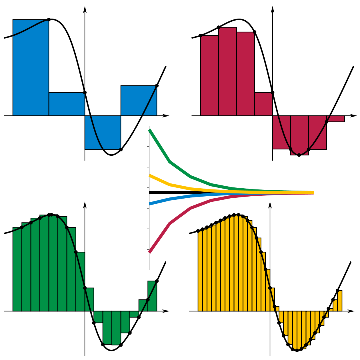
Draw the speed against time. Each little product "speed × time slice" is the area of a thin rectangle under the graph, so the total distance is the area under the speed curve.
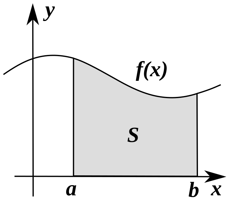
That is the general picture. To find the area under f between a and b:
- Cut [a,b] into n strips, each of width \Delta x = \frac{b-a}{n}.
- On each strip, build a rectangle of height f(x_i) for some point x_i in that strip.
- Add the areas: \sum_{i=1}^n f(x_i)\Delta x.
- Let n grow without bound.
\int_a^b f(x)\,dx = \lim_{n\to\infty}\sum_{i=1}^n f(x_i)\,\Delta x
This is the Riemann integral, and step 3's expression is a Riemann sum. The symbol \sum means "add up all of these"; if it is unfamiliar, read \sum_{i=1}^{n} as "add the following for i = 1 up to n".
The notation is Leibniz's and it is a picture in itself. The \int is an elongated S for summa, a sum. The dx is the infinitesimally thin width of a strip. So \int f(x)\,dx reads literally as "sum of height times width", which is what it is.
Signed area. Where f is below the axis the rectangles have negative height, so their contribution is negative. \int_0^{2\pi}\sin x\,dx = 0, because the hump above the axis exactly cancels the hump below. If you want the geometric area regardless of sign, integrate |f(x)|.
2. Computing one from the definition, once
Find \int_0^1 x^2\,dx from first principles, so you can see what the machinery of Section 3 saves you.
Cut [0,1] into n strips of width \frac{1}{n}, taking the height at the right end of each strip, so x_i = \frac{i}{n}:
S_n = \sum_{i=1}^n \left(\frac{i}{n}\right)^2\cdot\frac{1}{n} = \frac{1}{n^3}\sum_{i=1}^n i^2
There is a known formula for the sum of the first n squares:
\sum_{i=1}^n i^2 = \frac{n(n+1)(2n+1)}{6}
So:
S_n = \frac{n(n+1)(2n+1)}{6n^3} = \frac{2n^3 + 3n^2 + n}{6n^3} = \frac{1}{3} + \frac{1}{2n} + \frac{1}{6n^2}
As n\to\infty the last two terms vanish (Chapter 5.1):
\int_0^1 x^2\,dx = \frac{1}{3}
That was a lot of work for one simple integral, and it needed a special summation formula. Doing it for \sin x or e^x would be far worse. This is exactly the situation calculus was in before the next section.
The argument above claimed that thinner rectangles close in on the true area. Here it is happening, with the error shown as a number.
estimate = 1.75true value = 2.666667error = -0.916667width h = 0.5
The important thing is not that the error shrinks but how it shrinks. Doubling n roughly halves the left-corner error, while the midpoint and trapezoid rules improve four times faster for the same work. That difference is what Part 10 is built on.
3. The Fundamental Theorem of Calculus
Newton and Leibniz independently found the connection, and it is the reason both are remembered. Areas had been computed for two thousand years by exhausting arguments like the one above, one shape at a time. Tangents had been studied separately. Nobody had noticed the two problems were inverses of each other.
Part 1. Define a function by accumulating area from a fixed start:
F(x) = \int_a^x f(t)\,dt
Then
F'(x) = f(x)
The derivative of the accumulated area is the height of the curve. The reason is visible: extend the region by a sliver of width dx and you add area f(x)\,dx, so the rate of area growth is f(x).
Part 2, which is the one you compute with. If F is any function whose derivative is f, then
\int_a^b f(x)\,dx = F(b) - F(a)
To find an area, find any antiderivative and subtract its values at the two ends. No sums, no limits.
Redo the earlier example. An antiderivative of x^2 is \frac{x^3}{3}, since differentiating it gives x^2. So:
\int_0^1 x^2\,dx = \left[\frac{x^3}{3}\right]_0^1 = \frac{1}{3} - 0 = \frac{1}{3}
One line instead of a page, and the same answer. That is what the theorem buys, and it is why calculus transformed science within a generation of its discovery.
The square-bracket notation with limits means "evaluate at the top, subtract the value at the bottom".
4. Antiderivatives and the constant
An antiderivative of f is any function whose derivative is f. They are never unique: if F' = f then (F + C)' = f too for any constant, since constants differentiate to zero.
The indefinite integral collects them all:
\int f(x)\,dx = F(x) + C
The +C is not pedantry. It is the statement that knowing a rate does not tell you a starting value. Knowing your speed for an hour tells you how far you travelled, not where you are — for that you need to know where you began. In a differential equation (Chapter 6.1) the constant is fixed by an initial condition, and getting it wrong is getting the answer wrong.
The standard antiderivatives, each just a derivative rule from Chapter 5.3 read backwards:
\int x^n dx = \frac{x^{n+1}}{n+1} + C \quad (n\neq-1) \qquad \int \frac{1}{x}dx = \ln|x| + C
\int e^x dx = e^x + C \qquad \int \sin x\,dx = -\cos x + C \qquad \int\cos x\,dx = \sin x + C
The exception at n = -1 exists because the power rule would give \frac{x^0}{0}, dividing by zero. That gap is exactly where the logarithm lives, which is a rather satisfying piece of bookkeeping: the one power the rule cannot handle is the one that needs a different kind of function entirely. The absolute value in \ln|x| handles negative x, where the logarithm itself is undefined but the reciprocal is not.
5. What integrals compute besides area
Area is where the idea comes from. Almost every use is something else.
Distance from speed, the opening example: s = \int v\,dt.
Volume by slicing. Cut a solid into thin discs perpendicular to an axis; each disc has volume \pi r(x)^2\,dx, and integrating gives the total. For a sphere of radius R, a slice at height x is a disc of radius \sqrt{R^2-x^2}:
V = \int_{-R}^{R}\pi(R^2-x^2)\,dx = \pi\left[R^2x - \frac{x^3}{3}\right]_{-R}^{R} = \pi\left(\frac{2R^3\cdot 2}{3}\right)\cdot\frac{1}{2}\cdot 2 = \frac{4}{3}\pi R^3
Archimedes' result from Chapter 3.3, in three lines, using a method he did not have.
Work done by a varying force: W = \int F\,dx. Compressing a spring takes more force as it compresses, so the total work is an integral.
Average value of a function over an interval:
\bar f = \frac{1}{b-a}\int_a^b f(x)\,dx
which is the continuous version of "add them up and divide by how many".
This is how mains voltage is quoted. A sine wave averages zero over a cycle, so the useful average is the root mean square — square it (making everything positive), average, then take the root:
V_{\text{rms}} = \sqrt{\frac{1}{T}\int_0^T V_0^2\sin^2(\omega t)\,dt} = \frac{V_0}{\sqrt2}
So "230 volts" means the RMS value, and the actual peak is 230\sqrt2 = 325 volts. That peak is what a component's insulation must withstand, which is why the distinction is not academic.
Probability. For a continuous random variable, the probability of landing in a range is the area under the density curve over that range, and the total area is 1. Chapter 7.4 develops it.
Centre of mass, moment of inertia, arc length, surface area, total charge, total heat. All integrals. Anything that is a total of continuously varying contributions is an integral.
6. Improper integrals: infinite regions with finite area
What is \int_1^\infty \frac{1}{x^2}dx? The region extends forever to the right.
Compute up to a finite limit, then let the limit grow:
\int_1^b \frac{1}{x^2}dx = \left[-\frac{1}{x}\right]_1^b = 1 - \frac{1}{b} \;\longrightarrow\; 1
An infinitely long region with an area of exactly 1. The tail thins fast enough that the total stays finite, exactly as Zeno's halving distances did in Chapter 5.1.
Now \int_1^\infty\frac{1}{x}dx:
\left[\ln x\right]_1^b = \ln b \;\longrightarrow\; \infty
This one is infinite. The two curves look similar and behave completely differently, and the boundary between converging and diverging sits exactly at the power -1.
This is the same boundary that decides whether an infinite sum converges, and it is why the harmonic series 1 + \frac12 + \frac13 + \cdots adds up to infinity while 1 + \frac14 + \frac19 + \cdots does not. Chapter 5.8 pursues it.
Gabriel's Horn
Rotate y = \frac 1x for x \ge 1 about the horizontal axis. The solid you get has finite volume (\pi, exactly) and infinite surface area.
So it can be filled with a finite amount of paint, and yet you could never paint its inside surface.
The apparent paradox dissolves once you notice that "painting" means a coat of some fixed thickness, and near the far end the horn is thinner than any coat you could apply. Filling it with paint of no thickness is a different operation from painting it. Torricelli found this in 1641 and it caused a genuine philosophical uproar.
Every formula above, built from scratch
None of the results in this chapter are worth memorising, because each one can be rebuilt in under a minute from something simpler. What follows is that rebuilding, one result at a time, so the formula and the reason for it sit on the same page as the explanation that needed them.
The integral
\int_a^b f(x)\,dx = \lim_{n\to\infty}\sum_{i=1}^{n}f(x_i)\Delta x
Read it aloud. "The integral from a to b of f of x dee x" — the limit of a sum of rectangle areas as the rectangles become infinitely thin. The \int is a stretched letter S, for summa, and the dx records the width of each strip.
estimate = 1.75true value = 2.666667error = -0.916667width h = 0.5
The fundamental theorem of calculus
\frac{d}{dx}\int_a^x f(t)\,dt = f(x) \qquad\text{and}\qquad \int_a^b f(x)\,dx = F(b)-F(a) \text{ where } F' = f
Where the first part comes from — and it is the most important argument in this Part. Let A(x) be the area under the curve from a up to x. Now push the right edge along by a tiny amount h. The extra area is a sliver: it is almost a rectangle of width h and height f(x), and the error is a thin sliver of a sliver.
A(x+h) - A(x) \approx f(x)\cdot h
Divide by h:
\frac{A(x+h)-A(x)}{h} \approx f(x)
The left-hand side is exactly the difference quotient whose limit defines A'(x). Let h\to0 and the approximation becomes exact:
A'(x) = f(x)
The rate at which area accumulates is the height of the curve. That is the whole theorem in one sentence, and the second part follows: if F is any function whose derivative is f, then F and A differ by a constant, and that constant cancels in the subtraction F(b)-F(a).
This is why integration is done by running differentiation backwards, and why a problem about accumulated area is solved by a table of derivatives read from right to left.
Properties of definite integrals
\int_a^b = -\int_b^a, \qquad \int_a^a = 0, \qquad \int_a^b = \int_a^c + \int_c^b
\int_a^b (f+g) = \int_a^b f + \int_a^b g, \qquad \int_a^b cf = c\int_a^b f
Average value:
\bar f = \frac{1}{b-a}\int_a^b f(x)\,dx
Total accumulation divided by the width — the same idea as an ordinary average, with the sum replaced by an integral.
The complete integral table
Every line is a line of the derivative table, read backwards. The +C is compulsory: many functions share the same derivative, differing only by a constant, and the constant cannot be recovered from the derivative.
| \int f(x)\,dx | Result |
|---|---|
| \int x^n dx | \frac{x^{n+1}}{n+1}+C (for n\ne-1) |
| \int \frac1x dx | \ln\lvert x\rvert + C |
| \int e^x dx | e^x + C |
| \int a^x dx | \frac{a^x}{\ln a}+C |
| \int \sin x\,dx | -\cos x + C |
| \int \cos x\,dx | \sin x + C |
| \int \sec^2x\,dx | \tan x + C |
| \int \tan x\,dx | -\ln\lvert\cos x\rvert + C |
| \int \frac{dx}{\sqrt{1-x^2}} | \arcsin x + C |
| \int \frac{dx}{1+x^2} | \arctan x + C |
| \int \frac{dx}{x^2-a^2} | \frac{1}{2a}\ln\left\lvert\frac{x-a}{x+a}\right\rvert + C |
| \int \sinh x\,dx | \cosh x + C |
| \int \cosh x\,dx | \sinh x + C |
| \int \ln x\,dx | x\ln x - x + C |
Why the power rule needs the exception. \frac{x^{n+1}}{n+1} divides by n+1, which is zero when n = -1. The gap is filled by the logarithm, exactly as §2 predicted.
Why \int\tan x\,dx is a logarithm. Write \tan x = \frac{\sin x}{\cos x} and substitute u = \cos x, so du = -\sin x\,dx:
\int\frac{\sin x}{\cos x}dx = -\int\frac{du}{u} = -\ln|u| + C = -\ln|\cos x| + C
Where \int\ln x\,dx comes from — by parts, taking u = \ln x and dv = dx:
\int \ln x\,dx = x\ln x - \int x\cdot\frac1x dx = x\ln x - x + C
Applications of the integral
\text{Area between curves} = \int_a^b \left(f(x)-g(x)\right)dx \quad (\text{upper minus lower})
\text{Volume of revolution, discs}: V = \pi\int_a^b \left[f(x)\right]^2dx
Where it comes from. Slice the solid perpendicular to the axis. Each slice is a disc of radius f(x) and thickness dx, so its volume is \pi r^2\,dx = \pi f(x)^2dx. Add them all up.
\text{Volume, shells}: V = 2\pi\int_a^b x f(x)\,dx
Each shell is a thin cylinder unrolled into a rectangle: height f(x), width 2\pi x (the circumference at radius x), thickness dx.
\text{Arc length}: L = \int_a^b\sqrt{1+\left(\frac{dy}{dx}\right)^2}\,dx
Where it comes from. A tiny piece of the curve is nearly straight, so by Pythagoras its length is \sqrt{(dx)^2+(dy)^2}. Factor out dx:
\sqrt{(dx)^2\left(1 + \left(\tfrac{dy}{dx}\right)^2\right)} = \sqrt{1+\left(\tfrac{dy}{dx}\right)^2}\,dx
\text{Surface of revolution}: S = 2\pi\int_a^b f(x)\sqrt{1+(f'(x))^2}\,dx
Each band is a strip of length ds swept around a circle of circumference 2\pi f(x).
7. Where this shows up in your life
Every distance-from-speed and total-from-rate calculation. Odometers, fuel gauges, electricity meters, data usage counters.
Every electricity bill. Energy is the integral of power over time, and the meter on your wall is an integrator.
Every probability quoted from a distribution. The area under the curve.
Every engineering stress calculation. Total force on a dam wall from pressure that increases with depth is an integral.
Every medical dose calculation. The "area under the curve" of drug concentration against time is the standard measure of total exposure, and it is literally an integral.
Every image and audio processing operation. Blurring is an integral of nearby values; Chapter 9.4 explains it as convolution.
Every mains-powered device. The RMS calculation of Section 5.
Differentiating any function you can write down is mechanical. Integrating is not, and the next chapter is honest about why — along with the techniques that handle the cases that can be done.