Appearance
2.2 — Damping and Resonance
On 7 November 1940 the Tacoma Narrows Bridge in Washington State twisted itself apart in a 68 km/h wind. Not a storm — a moderate breeze, well under half what the bridge was designed for. It had been open four months. Film of the collapse shows the deck rolling through an angle of nearly 45°, one lane rising as the other falls, over and over, for about an hour before it tore.
A steady wind is not oscillating. The bridge was. Understanding how a constant input becomes a growing oscillation is what this chapter is for, and it is the same mechanism that lets a radio pick one station out of hundreds and lets an MRI scanner see inside you.
Damping: where the energy goes
Chapter 2.1's oscillator runs forever, because nothing takes energy out. Real ones have friction, air resistance, and internal losses in the material as it flexes.
For an object moving through a fluid at modest speed, the resisting force is proportional to velocity:
F_{\text{damp}} = -bv = -b\frac{dx}{dt}
where b is the damping coefficient in newton-seconds per metre. The minus sign says it always opposes the motion. (Chapter 1.11's v^2 drag applies at higher speeds; the linear form is the one that keeps the mathematics solvable, and it is a good model for a shock absorber, for a mass in oil, and for the electrical resistance in a circuit.)
Newton's second law now has two forces:
m\frac{d^2x}{dt^2} = -kx - b\frac{dx}{dt}
Rearranged into standard form:
\boxed{\frac{d^2x}{dt^2} + \frac{b}{m}\frac{dx}{dt} + \frac{k}{m}x = 0}
Define two symbols that will be used for the rest of the chapter:
\omega_0 = \sqrt{\frac{k}{m}} \quad\text{(the undamped natural frequency)}, \qquad \gamma = \frac{b}{2m} \quad\text{(the damping rate)}
\frac{d^2x}{dt^2} + 2\gamma\frac{dx}{dt} + \omega_0^2x = 0
Solving it
The standard method for a linear equation with constant coefficients (Volume II, Chapter 6.3) is to try x = e^{\lambda t}, because the exponential is the one function whose derivatives are all copies of itself. Substituting gives \lambda^2e^{\lambda t} + 2\gamma\lambda e^{\lambda t} + \omega_0^2e^{\lambda t} = 0, and dividing out the never-zero e^{\lambda t} leaves an ordinary quadratic:
\lambda^2 + 2\gamma\lambda+\omega_0^2 = 0
\lambda = \frac{-2\gamma \pm \sqrt{4\gamma^2-4\omega_0^2}}{2} = -\gamma \pm\sqrt{\gamma^2-\omega_0^2}
Everything now depends on the sign of what is under the square root, and that gives the three cases.
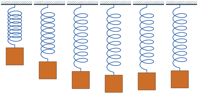
Case 1: light damping, \gamma < \omega_0
The square root is of a negative number, so it is imaginary. Write \sqrt{\gamma^2-\omega_0^2} = i\omega_d where
\omega_d = \sqrt{\omega_0^2-\gamma^2}
Then \lambda = -\gamma \pm i\omega_d, and using Euler's formula (Volume II, Chapter 2.5) the real solution is:
\boxed{x(t) = Ae^{-\gamma t}\sin(\omega_dt+\phi)}
An oscillation, with an amplitude that dies away exponentially. Three things to read off it:
The amplitude envelope is Ae^{-\gamma t}. Every cycle is a fixed fraction of the one before, not a fixed amount smaller. So the decay is fast at first and then drags on.
The energy decays twice as fast as the amplitude, since E \propto A^2:
E(t) = E_0e^{-2\gamma t}
The frequency is slightly lowered, from \omega_0 to \sqrt{\omega_0^2-\gamma^2}. For light damping the shift is tiny — with \gamma = 0.1\omega_0 it is only 0.5% — which is why a slowly dying pendulum still keeps good time.
Case 2: critical damping, \gamma = \omega_0
The square root is exactly zero, so the two roots coincide at \lambda = -\gamma. A repeated root needs a second solution of the form te^{\lambda t} (this is the standard rule for repeated roots; substituting it into the equation and using \gamma = \omega_0 shows it works):
x(t) = (A+Bt)e^{-\gamma t}
No oscillation at all. The system returns to equilibrium and stops. Critical damping is the fastest possible return to equilibrium without overshooting, and that makes it the target for an enormous amount of engineering.
Car shock absorbers are set close to critical. Under-damp them and the car bounces for several cycles after every bump; over-damp them and the wheel cannot follow the road surface, so grip is lost. Manufacturers usually pick slightly under critical, around \gamma = 0.7\omega_0, which returns almost as fast and feels less harsh.
The same target governs the needle on an analogue meter (which should swing straight to the reading and stop), a door closer (which should shut the door firmly without slamming or bouncing), and the servo positioning a hard drive's read head.
Case 3: heavy damping, \gamma > \omega_0
The square root is real, so both roots are real and negative:
x(t) = Ae^{-(\gamma-\sqrt{\gamma^2-\omega_0^2})t} + Be^{-(\gamma+\sqrt{\gamma^2-\omega_0^2})t}
A slow crawl back to equilibrium with no oscillation, and slower than critical damping — this is the counter-intuitive part. Adding more damping past the critical point makes the return worse, because the resistance now fights the return itself. A door closer screwed too tight takes a minute to shut the door.
| Case | Condition | Behaviour | Example |
|---|---|---|---|
| Light | \gamma<\omega_0 | Oscillates, decays | Guitar string, pendulum |
| Critical | \gamma=\omega_0 | Fastest return, no overshoot | Meter needle, door closer |
| Heavy | \gamma>\omega_0 | Slow return, no overshoot | Very thick oil, tight door closer |
The quality factor
How lightly damped a system is gets one number:
Q = \frac{\omega_0}{2\gamma} = 2\pi\times\frac{\text{energy stored}}{\text{energy lost per cycle}}
High Q means low loss and a long ring. The number of oscillations before the amplitude falls to about 4% of its start is roughly Q itself, which makes it easy to estimate by watching.
| System | Q |
|---|---|
| Car suspension | ~1 |
| Simple pendulum in air | ~10³ |
| Guitar string | ~10³ |
| Quartz watch crystal | ~10⁵ |
| Caesium atomic clock | ~10⁸ |
| LIGO's test masses | ~10⁹ |
That last one is why gravitational-wave detection is possible at all: the mirrors are suspended so cleanly that they ring for years, and Chapter 6.10 explains what is being measured.
Driven oscillation and resonance
Now push the oscillator with a periodic force at your own chosen frequency \omega, which need not match the system's \omega_0:
m\frac{d^2x}{dt^2} = -kx - b\frac{dx}{dt} + F_0\cos(\omega t)
\frac{d^2x}{dt^2}+2\gamma\frac{dx}{dt}+\omega_0^2x = \frac{F_0}{m}\cos(\omega t)
After the initial transient dies away — which takes a few multiples of 1/\gamma — the system settles into oscillating at the driving frequency, not its own. That is worth stating clearly, because it is the first surprise: push a swing at any rhythm you like and eventually it moves at your rhythm, not its natural one.
Assume the settled solution x = A\cos(\omega t - \delta), where \delta is how far the response lags the push. Substituting and solving (the algebra is a standard trigonometric-identity grind, and the result is what matters) gives:
\boxed{A(\omega) = \frac{F_0/m}{\sqrt{(\omega_0^2-\omega^2)^2+4\gamma^2\omega^2}}}
\tan\delta = \frac{2\gamma\omega}{\omega_0^2-\omega^2}
Reading the amplitude formula
Everything about resonance is in the denominator, because a small denominator means a large amplitude.
Driving very slowly (\omega \to 0). The denominator becomes \omega_0^2, so A \to F_0/(m\omega_0^2) = F_0/k. The system just follows the force, as a spring would if you pushed it slowly by hand. It moves in phase with the push, \delta \to 0.
Driving very fast (\omega \gg \omega_0). The denominator is dominated by \omega^4 under the root, so A \to F_0/(m\omega^2), which goes to zero. The mass cannot keep up; its inertia wins. It moves exactly out of phase, \delta \to \pi — you push right and it is moving left.
Driving near \omega_0. The first term in the denominator, (\omega_0^2-\omega^2)^2, collapses towards zero. All that survives is 4\gamma^2\omega^2, the damping term, and if damping is small the denominator is tiny and the amplitude is enormous.
A_{\text{res}} \approx \frac{F_0}{2m\gamma\omega_0} = \frac{F_0Q}{k}
The amplitude at resonance is Q times the static displacement. A system with Q = 1000 driven at its natural frequency moves a thousand times further than the same force applied steadily. That is the whole phenomenon in one line.
The peak is not exactly at \omega_0. Differentiating the denominator and setting it to zero gives:
\omega_{\text{res}} = \sqrt{\omega_0^2-2\gamma^2}
slightly below the natural frequency, and below the damped frequency \omega_d as well. For light damping all three are indistinguishable.
At resonance the phase lag is exactly \delta = \pi/2 — a quarter cycle behind — and that is the mechanism. A quarter-cycle lag means the driving force is always in the same direction as the velocity. Since power delivered is \vec{F}\cdot\vec{v} from Chapter 1.6, the force is doing positive work at every single instant of every cycle. Energy only ever goes in. At any other frequency the force spends part of each cycle opposing the motion and takes some energy back out.
That is also exactly what you do when pushing a child on a swing. You push when they are moving away from you — in phase with velocity, not with position — and each push adds a little. Push at the wrong moment and you take energy out, which is how you stop the swing.
Sharpness
The resonance peak's width at the points where the power is half its maximum is:
\Delta\omega = 2\gamma \quad\Longrightarrow\quad \frac{\omega_0}{\Delta\omega} = Q
High Q means a tall, narrow peak; low Q means a low, broad one. So Q measures two things at once — how long it rings and how selective it is — and they are the same property seen from two sides.
Selectivity is exactly what a radio tuner needs. A tuned circuit with Q = 100 at 100 MHz has a bandwidth of 1 MHz, wide enough to pass one FM station's signal and narrow enough to reject its neighbours 0.2 MHz away. Volume III, Chapter 1.6 builds that circuit.
Where resonance is useful and where it is a disaster
Useful:
- Musical instruments. A guitar body, a violin's air cavity and an organ pipe are all resonators that amplify the string's or reed's vibration into something audible. A solid-body electric guitar deliberately has no resonant cavity, which is why it is nearly silent unamplified.
- Radio and every wireless thing you own. Tuning is choosing \omega_0 to match the station.
- Microwave ovens. Often explained as hitting a resonance of the water molecule, which is not right — water's rotational resonances are much higher and much sharper. A microwave oven at 2.45 GHz works by dielectric heating: the field flips 2.45 billion times a second and drags the polar water molecules round with it, and they lose energy to their neighbours as they turn. The frequency is chosen for penetration depth and for being an allocated band, not for a resonance.
- MRI. Nuclear magnetic resonance is a genuine resonance: protons in a strong magnetic field precess at a frequency proportional to the field, and a radio pulse at exactly that frequency tips them. Because the frequency depends on the field, applying a field that varies across the body lets each slice be addressed separately. Chapter 7.7 covers the spin physics.
- Atomic clocks. The caesium transition of Chapter 1.1 is a resonance with Q \approx 10^8, which is why it defines the second.
Disastrous:
- Tacoma Narrows. The usual telling calls it simple forced resonance, and that is not quite what happened. The deck's own twisting motion changed how the air flowed past it, which changed the force, which fed the twisting. That is aeroelastic flutter — a self-driven oscillation where the structure sets its own driving frequency — and it is more dangerous than plain resonance because there is no external frequency to avoid. Every long bridge since is wind-tunnel tested for it, and modern decks have open gaps and aerofoil profiles specifically to stop the airflow locking onto the motion.
- The Millennium Bridge, London, 2000. It opened, wobbled sideways, and closed after two days. Pedestrians naturally adjust their gait to keep balance on a moving surface, so they unconsciously synchronised with the bridge's 1 Hz lateral mode and drove it. Nobody had modelled the crowd as part of the system. The fix was 37 dampers, and the physics is now called synchronous lateral excitation.
- Soldiers break step on bridges for exactly this reason, and have done since a suspension bridge at Broughton collapsed under marching troops in 1831.
- Buildings in earthquakes. A building's natural period is roughly N/10 seconds for N storeys, so a ten-storey building rings at about 1 Hz — which is squarely in the band that earthquakes deliver most energy. Tall buildings therefore carry tuned mass dampers: a large mass on springs, tuned to the building's own frequency and deliberately damped, so it oscillates out of phase and absorbs the energy. Taipei 101 has a 660-tonne steel sphere hanging in its upper floors, and it is a tourist attraction.
- The wine glass. A crystal glass has a high-Q ringing mode you can hear by tapping it. Drive it at that frequency loudly enough and the rim's amplitude grows until the strain exceeds what glass can take — and glass is brittle, so it goes suddenly, exactly as Chapter 1.10 described. It needs a genuinely loud, genuinely on-pitch note; most attempts fail because being 1% off frequency on a Q = 1000 system loses most of the gain.
Worked example: a tuned mass damper
A footbridge has a natural frequency of 2.0 Hz and Q = 50. Walking pedestrians deliver a rhythmic force of 40 N amplitude. The bridge's effective stiffness is 2.0\times10^6\ \text{N/m}. How far does it move at resonance, and how much does adding damping to bring Q down to 5 help?
Static deflection under 40 N:
x_{\text{static}} = \frac{F_0}{k} = \frac{40}{2.0\times10^6} = 2.0\times10^{-5}\ \text{m} = 0.02\ \text{mm}
Two hundredths of a millimetre. Invisible.
At resonance:
A = Qx_{\text{static}} = 50\times0.02 = 1.0\ \text{mm}
A millimetre of sway at 2 Hz is enough for people to feel and to find unsettling.
With dampers bringing Q to 5:
A = 5\times0.02 = 0.1\ \text{mm}
Worth noticing. The force never changed. Nothing was strengthened. All that changed was how much of each cycle's energy is thrown away, and the motion dropped by a factor of ten. Fixing a resonance problem is almost always about adding damping or moving the frequency, and almost never about adding strength — a stiffer bridge has a higher natural frequency, which may move it out of the pedestrian band or may move it straight into another one.
Where this shows up in your life
Your washing machine shakes violently at one particular speed during the spin-up and then settles down once it is faster. That speed is the resonance of the drum-on-springs system, and the machine passes through it on the way to its running speed. Modern machines detect the load imbalance and ramp through that band quickly rather than dwelling in it.
Every car has a speed at which some trim panel buzzes and no other speed at which it does. The engine and road deliver a broad range of frequencies; the panel has one natural frequency and picks its own out of the mixture. The fix — a piece of foam — is damping, not stiffening.
And the reason you can hear a specific pitch at all is that your inner ear is a bank of resonators. The basilar membrane in the cochlea varies in stiffness and width along its length, so each position has its own natural frequency, from about 20 kHz at one end to 20 Hz at the other. A sound sets one region moving more than the rest, and the nerve cells there report it. Hearing is Fourier analysis done with mechanical resonance, and Chapter 2.4 makes that connection precise.
What the next chapter fixes
An oscillator so far sits in one place and moves. But if you have a row of them, each connected to its neighbour, then disturbing one disturbs the next a moment later, and the disturbance travels. That travelling disturbance is a wave, and it is what sound, light, earthquakes and quantum particles all turn out to be. Chapter 2.3 derives the wave equation from a stretched string, using nothing but Newton's second law applied to a small curved piece of it.