Appearance
4.7 — Maxwell's Equations and the Discovery of Light
Four laws are now on the table. Write them together:
\oint\vec{E}\cdot d\vec{A} = \frac{Q}{\varepsilon_0} \qquad\text{(Gauss, Chapter 4.2)}
\oint\vec{B}\cdot d\vec{A} = 0 \qquad\text{(no monopoles, Chapter 4.5)}
\oint\vec{E}\cdot d\vec{l} = -\frac{d\Phi_B}{dt} \qquad\text{(Faraday, Chapter 4.6)}
\oint\vec{B}\cdot d\vec{l} = \mu_0I \qquad\text{(Ampère, Chapter 4.5)}
James Clerk Maxwell looked at this set in the early 1860s and noticed that the fourth one is wrong — not approximately, not in some exotic regime, but flatly self-contradictory in an experiment anyone could do with a battery and two metal plates. Fixing it required adding one term, and the fixed set turned out to predict something nobody was looking for.

The contradiction in Ampère's law
Ampère's law says: take any closed loop, add up \vec{B}\cdot d\vec{l} around it, and the answer is \mu_0 times the current passing through the loop.
"Through the loop" needs care. A loop is a curve; a current passes through a surface bounded by that curve. And there are infinitely many surfaces with the same boundary — think of a soap film on a wire ring, which you can blow into any shape you like without moving the ring.
Ampère's law is only consistent if every one of those surfaces gives the same answer. For steady currents in complete circuits it does, because current is conserved and whatever flows through one surface flows through any other with the same rim.
Now charge a capacitor.
Current I flows along the wire towards one plate. Draw a circular loop around that wire. Now choose two surfaces bounded by it:
- Surface 1: a flat disc, cutting straight through the wire. Current through it: I. Ampère's law gives \oint\vec{B}\cdot d\vec{l} = \mu_0I.
- Surface 2: a bag-shaped surface with the same circular rim, bulging out sideways and passing between the capacitor plates. No charge crosses the gap — that is what a capacitor is. Current through it: zero. Ampère's law gives \oint\vec{B}\cdot d\vec{l} = 0.
Same loop, same magnetic field around it, two different answers. Ampère's law as written is broken.
Maxwell's fix
Something must be crossing the gap in the second surface, and Maxwell asked what is going on there that is not going on in the wire.
The answer: the electric field between the plates is growing. Charge is accumulating on the plates, so from Chapter 4.2 the field E = \sigma/\varepsilon_0 = Q/\varepsilon_0A is rising in step.
Compute how fast the flux of that field is rising:
\Phi_E = EA = \frac{Q}{\varepsilon_0A}\cdot A = \frac{Q}{\varepsilon_0}
\frac{d\Phi_E}{dt} = \frac{1}{\varepsilon_0}\frac{dQ}{dt} = \frac{I}{\varepsilon_0}
Rearranged:
I = \varepsilon_0\frac{d\Phi_E}{dt}
The rate of change of electric flux through the gap is numerically equal to the current in the wire. Exactly equal, not approximately. So if this quantity is added to Ampère's law as though it were a current, both surfaces give the same answer, and the contradiction disappears.
\boxed{\oint\vec{B}\cdot d\vec{l} = \mu_0\left(I + \varepsilon_0\frac{d\Phi_E}{dt}\right)}
Maxwell called the new term the displacement current. The name is a leftover from a mechanical model of the ether that he later abandoned, and it is misleading: nothing is displaced and no charge flows. What the term says is:
A changing electric field produces a magnetic field, exactly as a real current does.
This completes a symmetry. Faraday had shown that a changing \vec{B} makes an \vec{E}. Maxwell now says a changing \vec{E} makes a \vec{B}. Neither needs any matter to be present.
Was this a guess? Partly. Maxwell had no experimental evidence for the term — the effect is far too small to detect in an ordinary charging capacitor. He added it because the equations were inconsistent without it and because the symmetry appealed to him. He was right, and it is one of the great examples in physics of theoretical consistency leading to a real discovery.
The four equations
\oint\vec{E}\cdot d\vec{A} = \frac{Q_{\text{enc}}}{\varepsilon_0}
\oint\vec{B}\cdot d\vec{A} = 0
\oint\vec{E}\cdot d\vec{l} = -\frac{d\Phi_B}{dt}
\oint\vec{B}\cdot d\vec{l} = \mu_0 I_{\text{enc}} + \mu_0\varepsilon_0\frac{d\Phi_E}{dt}
Read in plain English, one at a time:
1. Electric field lines begin and end on charges. The flux out of a closed surface counts the charge inside.
2. Magnetic field lines never begin or end. They form closed loops. There are no magnetic charges.
3. A changing magnetic field wraps an electric field around itself.
4. An electric current, or a changing electric field, wraps a magnetic field around itself.
Add the force law that says what the fields do to matter:
\vec{F} = q(\vec{E} + \vec{v}\times\vec{B})
and you have every electric, magnetic and optical phenomenon in nature, from a static shock to a radio broadcast to the colour of the sky. Everything in Volume III's Parts 7 and 8 is engineering built on these five lines.
The same equations in differential form
Physicists usually write them in a compact local form, which says the same thing about each point in space rather than about surfaces and loops:
\nabla\cdot\vec{E} = \frac{\rho}{\varepsilon_0}, \qquad \nabla\cdot\vec{B} = 0
\nabla\times\vec{E} = -\frac{\partial\vec{B}}{\partial t}, \qquad \nabla\times\vec{B} = \mu_0\vec{J} + \mu_0\varepsilon_0\frac{\partial\vec{E}}{\partial t}
Two new symbols, both explained in Volume II, Chapter 5.7, and both readable in words.
\nabla\cdot\vec{E} is the divergence: how much the field spreads out from a point, like water from a spring. It is positive where lines are being created and negative where they end.
\nabla\times\vec{E} is the curl: how much the field circulates around a point, like water going down a drain. It is what a tiny paddle wheel placed there would do.
So the four equations read: electric fields diverge from charge; magnetic fields never diverge; electric fields curl around changing magnetic fields; magnetic fields curl around currents and changing electric fields. The integral and differential forms are mathematically equivalent, connected by the divergence and Stokes theorems.
Deriving the wave
Now the payoff. Look at what the last two equations do in empty space — no charges, no currents, so \rho = 0 and \vec{J} = 0:
\nabla\times\vec{E} = -\frac{\partial\vec{B}}{\partial t}, \qquad \nabla\times\vec{B} = \mu_0\varepsilon_0\frac{\partial\vec{E}}{\partial t}
Each field is created by the other one changing. That is a feedback loop with no matter in it at all, and a feedback loop like this ought to be able to sustain itself.
Follow it through with a one-dimensional case, which keeps the calculus honest and readable. Suppose the electric field points along y and depends only on x and t, and the magnetic field points along z and likewise. For this geometry the curl equations reduce to:
\frac{\partial E_y}{\partial x} = -\frac{\partial B_z}{\partial t} \qquad (1)
-\frac{\partial B_z}{\partial x} = \mu_0\varepsilon_0\frac{\partial E_y}{\partial t} \qquad (2)
Step 1. Differentiate (1) with respect to x:
\frac{\partial^2 E_y}{\partial x^2} = -\frac{\partial}{\partial x}\frac{\partial B_z}{\partial t} = -\frac{\partial}{\partial t}\frac{\partial B_z}{\partial x}
Swapping the order of the two derivatives is allowed for any well-behaved field, and it is the step that makes the whole thing work.
Step 2. From (2), \partial B_z/\partial x = -\mu_0\varepsilon_0\,\partial E_y/\partial t. Substitute:
\frac{\partial^2 E_y}{\partial x^2} = -\frac{\partial}{\partial t}\left(-\mu_0\varepsilon_0\frac{\partial E_y}{\partial t}\right)
\boxed{\frac{\partial^2 E_y}{\partial x^2} = \mu_0\varepsilon_0\frac{\partial^2 E_y}{\partial t^2}}
Stop and look at that. Chapter 2.3 derived the wave equation from a piece of stretched string and it came out as:
\frac{\partial^2 y}{\partial x^2} = \frac{1}{v^2}\frac{\partial^2 y}{\partial t^2}
The two are the same equation. The electric field in empty space obeys a wave equation, with:
\frac{1}{v^2} = \mu_0\varepsilon_0 \quad\Longrightarrow\quad v = \frac{1}{\sqrt{\mu_0\varepsilon_0}}
The identical manipulation starting from (2) gives the same equation for B_z. So both fields propagate as waves, together, at the same speed.
The number
Now put the constants in. Both were measured in laboratories with no light involved anywhere.
\varepsilon_0 = 8.854\times10^{-12} C²N⁻¹m⁻², measured by charging capacitors and measuring forces between charges.
\mu_0 = 4\pi\times10^{-7} = 1.2566\times10^{-6} T m/A, measured by the force between two current-carrying wires.
\mu_0\varepsilon_0 = (1.2566\times10^{-6})(8.854\times10^{-12}) = 1.1127\times10^{-17}
v = \frac{1}{\sqrt{1.1127\times10^{-17}}} = \frac{1}{3.3357\times10^{-9}} = 2.998\times10^{8}\ \text{m/s}
Fizeau had measured the speed of light in 1849, by bouncing a beam off a distant mirror through the teeth of a spinning wheel, and got 3.15\times10^8 m/s. Foucault refined it to 2.98\times10^8.
Maxwell wrote, in 1865:
"This velocity is so nearly that of light, that it seems we have strong reason to conclude that light itself (including radiant heat, and other radiations if any) is an electromagnetic disturbance in the form of waves propagated through the electromagnetic field according to electromagnetic laws."
That is the discovery of what light is, and it came from measuring the force between two wires and the charge on two plates. Nobody had shone a light in the experiment.
Since the 2019 SI redefinition (Chapter 1.1) this has been turned around: c is defined as exactly 299,792,458 m/s and the metre is defined from it. So the relation c = 1/\sqrt{\mu_0\varepsilon_0} is now a definition of \varepsilon_0 rather than a prediction. The physics is unchanged; only the bookkeeping moved.
What the wave looks like
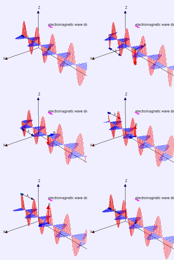
Four properties fall out of the derivation, and each has consequences.
1. It is transverse. Both fields point perpendicular to the direction of travel. Nothing oscillates along the direction of motion. This is why light can be polarised — there are two independent perpendicular directions available, and Chapter 5.5 develops it.
2. \vec{E} and \vec{B} are perpendicular to each other, and \vec{E}\times\vec{B} points in the direction of travel.
3. They are in phase. Both reach maximum at the same instant and zero at the same instant. This is worth stressing because it is different from a mechanical wave, where kinetic and potential energy are a quarter cycle apart. Here the two fields rise and fall together.
4. Their magnitudes are locked:
E = cB
which follows from equation (1) applied to a sinusoidal wave. Since c is large, E in volts per metre is always numerically about 3\times10^8 times B in tesla. Sunlight at the ground has E \approx 1000 V/m and B \approx 3\times10^{-6} T — smaller than the Earth's field, which is why nobody noticed light's magnetic component for centuries.
No medium
The derivation used \rho = 0 and \vec{J} = 0 — nothing there at all. The wave needs no medium.
This was very hard to accept in 1865, and physicists spent forty years looking for the medium anyway, calling it the luminiferous ether. Every wave anyone had ever met needed something to wave: sound needs air, water waves need water, a string wave needs a string. Chapter 6.1 tells the story of the search, the Michelson–Morley experiment that failed to find it, and what Einstein made of the failure.
The modern answer is that the field itself is the thing that waves. Space with a field in it is not empty in the relevant sense, and the field carries energy and momentum, which is as physical as anything gets.
Energy and momentum in the wave
From Chapter 4.3 the electric field holds energy at density \frac{1}{2}\varepsilon_0E^2, and from Chapter 4.6 the magnetic field holds B^2/2\mu_0. Check whether they are equal in a wave, using B = E/c and c^2 = 1/\mu_0\varepsilon_0:
u_B = \frac{B^2}{2\mu_0} = \frac{E^2/c^2}{2\mu_0} = \frac{E^2\mu_0\varepsilon_0}{2\mu_0} = \frac{1}{2}\varepsilon_0E^2 = u_E
Exactly equal, at every instant and every point. The total is:
u = \varepsilon_0E^2
The energy flow per unit area per second is given by the Poynting vector, named after John Henry Poynting:
\boxed{\vec{S} = \frac{1}{\mu_0}\vec{E}\times\vec{B}}
Its direction is the direction the energy is going, and its magnitude in W/m² is the intensity. For a sinusoidal wave the time-average is:
\bar{S} = \frac{E_0^2}{2\mu_0c}
Worked number. Sunlight at Earth's orbit delivers 1361 W/m² (Chapter 3.7). Solve backwards for the field strength:
E_0 = \sqrt{2\mu_0c\bar{S}} = \sqrt{2(1.2566\times10^{-6})(3\times10^{8})(1361)} = \sqrt{1.026\times10^{6}} = 1013\ \text{V/m}
A kilovolt per metre, oscillating 5\times10^{14} times a second.
Radiation pressure
Maxwell's equations also predict that light carries momentum:
p = \frac{U}{c}
so light striking a surface pushes on it. For a perfectly absorbing surface the pressure is S/c; for a perfect mirror it is doubled to 2S/c, because the light's momentum is reversed rather than merely stopped.
At Earth's orbit:
P_{\text{rad}} = \frac{1361}{3\times10^{8}} = 4.5\times10^{-6}\ \text{Pa}
Under five micropascals — about ten billionths of atmospheric pressure. Tiny, and not zero, and it is measurable and useful.
Solar sails work on it. IKAROS, launched by Japan in 2010, unfurled a 200 m² sail and was measurably accelerated by sunlight alone. LightSail 2 raised its orbit in 2019 using nothing else. The force on 200 m² is about a millinewton, which does nothing in a hurry and everything over months, since it never runs out of fuel.
Comet tails point away from the Sun, not backwards along the comet's path, and they do so on the outbound leg as well as the inbound one. Radiation pressure and the solar wind push the dust and ions away from the Sun regardless of which way the comet is travelling. Kepler noticed this in 1619 and guessed the cause correctly, two and a half centuries before Maxwell explained it.
Optical tweezers use a focused laser to trap and move single cells and bacteria, with forces of piconewtons. Arthur Ashkin's Nobel Prize in 2018 was for this.
And inside a star, radiation pressure is a major part of what holds it up against gravity — dominant in the most massive stars, and the reason there is an upper limit to how massive a star can be (Chapter 12.1).
The spectrum
The derivation put no limit on the wavelength. Any frequency is a solution, and they all travel at c in vacuum. What we call light is the tiny slice our eyes respond to.
| Band | Wavelength | Frequency | Photon energy |
|---|---|---|---|
| Radio | > 1 m | < 300 MHz | < 1 μeV |
| Microwave | 1 mm – 1 m | 0.3–300 GHz | μeV–meV |
| Infrared | 700 nm – 1 mm | 0.3–430 THz | meV–1.7 eV |
| Visible | 400–700 nm | 430–750 THz | 1.7–3.1 eV |
| Ultraviolet | 10–400 nm | 0.75–30 PHz | 3.1–124 eV |
| X-ray | 0.01–10 nm | 30 PHz–30 EHz | 124 eV–124 keV |
| Gamma | < 0.01 nm | > 30 EHz | > 124 keV |
They are all the same phenomenon. The only difference between the radio wave carrying your phone call and the gamma ray from a decaying nucleus is how fast the field oscillates — a factor of about 10^{19} in frequency, and nothing else. They obey the same four equations.
Heinrich Hertz confirmed all of this in 1887. He built a spark gap to make an oscillating current, and a small loop with its own gap several metres away, and saw a tiny spark jump in the loop whenever the transmitter fired. He measured the wavelength by finding standing-wave nodes in the room, measured the frequency from the circuit, multiplied them, and got the speed of light. He showed the waves reflect, refract and polarise exactly as light does.
Asked what use it was, Hertz replied: "It's of no use whatsoever. This is just an experiment that proves Maestro Maxwell was right." Within eight years Marconi was sending signals across water with the same apparatus, and Volume III, Part 7 is the engineering discipline that grew out of it.
Where this shows up in your life
Every wireless thing you own — WiFi at 2.4 and 5 GHz, Bluetooth, mobile data, GPS, car keys, contactless payment, the radio in the kitchen — is an antenna making charges oscillate so they radiate, and another antenna letting the arriving field push its charges around. Chapter 4.7 is the physics; Volume III, Part 8 is the engineering.
A microwave oven runs at 2.45 GHz, which drives water's electric dipoles (Chapter 4.1) to flip back and forth, and their friction against neighbours becomes heat. It is not a resonance of the water molecule, a claim which appears everywhere and is wrong — water's rotational resonances are in the tens of gigahertz. 2.45 GHz was chosen because it penetrates food to a useful depth and sits in an unlicensed band.
Your phone's screen, the sunlight on it, the heat from your hand, and the X-ray at the dentist are the same waves at different frequencies.
Radio telescopes see the universe in a band our eyes cannot, and every image of a black hole, a pulsar or the cosmic microwave background in Part 12 exists because these equations say the whole spectrum is out there.
What the next chapter fixes
The equations are complete for fields in vacuum. Inside matter they need one more ingredient, because materials respond to magnetic fields in three quite different ways — some are pushed out of fields, some are pulled in weakly, and a few are pulled in so strongly that they keep their magnetisation after the field is removed. That last group includes every permanent magnet, every transformer core and every hard disk. Chapter 4.8 explains where a magnet's field actually comes from, given that Chapter 4.5 established there are no magnetic charges anywhere.