Appearance
7.6 — The Hydrogen Atom, Solved
Hydrogen is the only atom that can be solved exactly, and solving it is the moment quantum mechanics stops being a set of clever arguments and becomes the foundation of chemistry.
Bohr got the energies right in 1913 by assuming things he could not justify (Chapter 7.1). Schrödinger's equation gives the same energies with no assumptions at all — and it gives far more: three quantum numbers falling out of the mathematics, the shapes of the orbitals, and the reason the periodic table has the shape it has.
Setting it up
One electron, charge -e, around one proton, charge +e. The potential is Coulomb's (Chapter 4.3):
V(r) = -\frac{ke^2}{r}
The three-dimensional time-independent Schrödinger equation:
-\frac{\hbar^2}{2m}\nabla^2\psi - \frac{ke^2}{r}\psi = E\psi
where \nabla^2 (the Laplacian) is the three-dimensional second-derivative operator.
Use spherical coordinates, because the potential depends only on r. The three coordinates are:
- r — distance from the nucleus.
- \theta (theta) — the polar angle, measured down from the z axis, running from 0 to \pi.
- \phi (phi) — the azimuthal angle around the z axis, running from 0 to 2\pi.
In these coordinates the Laplacian is unpleasant:
\nabla^2 = \frac{1}{r^2}\frac{\partial}{\partial r}\left(r^2\frac{\partial}{\partial r}\right)+\frac{1}{r^2\sin\theta}\frac{\partial}{\partial\theta}\left(\sin\theta\frac{\partial}{\partial\theta}\right)+\frac{1}{r^2\sin^2\theta}\frac{\partial^2}{\partial\phi^2}
It looks worse than it is. The first term is the radial part; the last two together are the angular part, and they are exactly the angular momentum operator \hat{L}^2 divided by -\hbar^2r^2. That structure is what lets the problem separate.
Separation of variables
Try:
\psi(r,\theta,\phi) = R(r)\,Y(\theta,\phi)
Substitute and divide by RY. Everything depending on r collects on one side and everything angular on the other, so both must equal a constant. Write it as \ell(\ell+1) — a choice that looks arbitrary now and pays off shortly.
Angular equation:
\left[\frac{1}{\sin\theta}\frac{\partial}{\partial\theta}\left(\sin\theta\frac{\partial}{\partial\theta}\right)+\frac{1}{\sin^2\theta}\frac{\partial^2}{\partial\phi^2}\right]Y = -\ell(\ell+1)Y
Radial equation:
-\frac{\hbar^2}{2m}\left[\frac{1}{r^2}\frac{d}{dr}\left(r^2\frac{dR}{dr}\right)\right]+\left[-\frac{ke^2}{r}+\frac{\hbar^2\ell(\ell+1)}{2mr^2}\right]R = ER
Note the extra term in the bracket, \hbar^2\ell(\ell+1)/2mr^2. It is the centrifugal barrier — the quantum version of the fact that a rotating object resists being pulled inwards. It is positive and grows as 1/r^2 near the origin, so it keeps electrons with \ell > 0 away from the nucleus.
Separate the angular part again
Y(\theta,\phi) = \Theta(\theta)\Phi(\phi)
The \phi equation is the easy one:
\frac{d^2\Phi}{d\phi^2} = -m_\ell^2\Phi \quad\Longrightarrow\quad \Phi(\phi) = e^{im_\ell\phi}
Now the first quantum number appears, forced by geometry. Going all the way round in \phi must return the same value, since \phi and \phi+2\pi are the same place:
e^{im_\ell(\phi+2\pi)} = e^{im_\ell\phi} \quad\Longrightarrow\quad e^{2\pi im_\ell} = 1
\boxed{m_\ell = 0,\pm1,\pm2,\dots}
An integer, because a wave must join up with itself. This is exactly the standing-wave argument of Chapter 7.2, now in an angle instead of along a string.
The \theta equation has acceptable solutions — finite everywhere, including at the poles — only when:
\boxed{\ell = 0,1,2,3,\dots \quad\text{and}\quad |m_\ell| \leq \ell}
The second quantum number, and the constraint linking them. The solutions are called associated Legendre functions, and combined with \Phi they give the spherical harmonics Y_\ell^{m_\ell}.
The radial part
The radial equation has solutions that stay finite at the origin and decay at infinity only for certain energies. Substituting u = rR and working through gives solutions of the form:
R_{n\ell}(r) = (\text{polynomial in }r)\times e^{-r/na_0}
and the condition for the polynomial to terminate — otherwise the function blows up at large r — is:
\boxed{n = \ell+1,\ \ell+2,\dots \quad\text{equivalently}\quad \ell \leq n-1}
The third quantum number.
And the energies:
\boxed{E_n = -\frac{mk^2e^4}{2\hbar^2n^2} = -\frac{13.606\ \text{eV}}{n^2}}
Exactly Bohr's result, obtained here with no arbitrary assumptions whatsoever.
The three quantum numbers
| Symbol | Name | Values | Determines |
|---|---|---|---|
| n | Principal | 1, 2, 3, … | Energy and overall size |
| \ell | Orbital angular momentum | 0 to n-1 | Shape |
| m_\ell | Magnetic | -\ell to +\ell | Orientation |
n sets the energy. E_n = -13.6/n^2 eV, and the average radius grows roughly as n^2a_0.
\ell sets the total angular momentum:
|\vec{L}| = \sqrt{\ell(\ell+1)}\,\hbar
Note it is \sqrt{\ell(\ell+1)}, not \ell. For \ell = 1, |\vec{L}| = \sqrt{2}\hbar = 1.414\hbar, not \hbar. Bohr's model had L = n\hbar, which is wrong on two counts: the wrong formula, and the wrong quantum number.
Historical letters for \ell, inherited from nineteenth-century spectroscopy where lines were classified by appearance:
| \ell | Letter | From |
|---|---|---|
| 0 | s | sharp |
| 1 | p | principal |
| 2 | d | diffuse |
| 3 | f | fundamental |
| 4 | g | (alphabetical from here) |
m_\ell sets the z-component:
L_z = m_\ell\hbar
Why only one component? Because [\hat{L}_x,\hat{L}_y] = i\hbar\hat{L}_z \neq 0 (Chapter 7.5). You can know the magnitude and one component; the other two are indefinite. The angular momentum vector is not pointing in a definite direction — it is smeared over a cone.
And this is why |\vec{L}| > L_z^{\max}. For \ell = 1, |\vec{L}| = 1.414\hbar while the largest L_z is 1\hbar. The vector can never point exactly along z, because that would mean L_x = L_y = 0 exactly, which the commutator forbids.
Bohr's ground state was wrong
Here is the sharpest disagreement between the two models, and it is worth stating plainly.
For n = 1, \ell can only be 0. So the hydrogen ground state has zero orbital angular momentum.
Bohr's model says L = 1\hbar for n=1 — the electron is going round in a circle.
The electron in the ground state is not orbiting. Its wavefunction is spherically symmetric and its angular momentum is exactly zero. The mental picture of a little planet going round is wrong, and it was wrong from the beginning, even though it produced the right energies.
Orbital shapes
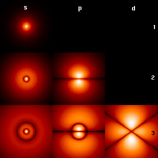
What the pictures actually show, because this is universally misunderstood:
They are probability clouds, not orbits. There is no path. The density at each point is |\psi|^2, the chance of finding the electron there if you look.
The usual textbook "boundary surface" is a 90 % contour. The wavefunction extends to infinity; the surface drawn encloses the region where the electron is found 90 % of the time. The choice of 90 % is arbitrary.
The colours in most diagrams show the sign of \psi, not charge. The wavefunction is positive in some lobes and negative in others, and that sign is essential — it determines whether two orbitals reinforce or cancel when atoms bond (Chapter 10.2). It has nothing to do with electric charge, which is negative everywhere.
s orbitals (\ell = 0)
Spherically symmetric. No angular dependence at all, since Y_0^0 is a constant.
The 1s wavefunction:
\psi_{1s} = \frac{1}{\sqrt{\pi a_0^3}}e^{-r/a_0}
Maximum probability density at r = 0 — the electron is most likely to be found at the nucleus, which surprises everybody.
But the most likely radius is a_0. These are different questions. The radial probability distribution — the chance of being in a shell between r and r+dr — includes the volume of the shell:
P(r) = 4\pi r^2|\psi|^2 = \frac{4r^2}{a_0^3}e^{-2r/a_0}
Maximise it:
\frac{dP}{dr} = \frac{4}{a_0^3}\left(2re^{-2r/a_0}-\frac{2r^2}{a_0}e^{-2r/a_0}\right) = 0 \quad\Longrightarrow\quad r = a_0
The most probable shell is at the Bohr radius. The density is highest at the origin; the shell volume there is zero. Both statements are true and they answer different questions.
Higher s orbitals have radial nodes. The 2s has one spherical surface where \psi = 0; the 3s has two. In general there are n-\ell-1 radial nodes.
p orbitals (\ell = 1)
Three of them, for m_\ell = -1, 0, +1, usually drawn as p_x, p_y, p_z — real combinations of the complex m_\ell states, which point along the axes and are more convenient for chemistry.
Dumbbell-shaped, two lobes along an axis with a nodal plane through the nucleus.
\psi_{2p_z} \propto r\cos\theta\,e^{-r/2a_0}
The electron has exactly zero probability of being at the nucleus, because of the factor r. This is the centrifugal barrier from the radial equation: any state with \ell > 0 is pushed away from the origin.
The two lobes have opposite signs of \psi, which is what makes p orbitals capable of forming directional bonds and is the whole reason molecules have shapes (Chapter 10.2).
d orbitals (\ell = 2) and f orbitals (\ell = 3)
Five d orbitals, four with a four-lobed cloverleaf shape and one (d_{z^2}) with two lobes and a doughnut around the middle. The odd one out is not a different kind of thing — it is a combination that happens to look different when drawn.
Seven f orbitals, with eight lobes and more complex nodal structure.
Angular nodes = \ell. s has none, p has one plane, d has two, f has three.

The total node count is always n-1, split between radial and angular. More nodes means more curvature means more kinetic energy (Chapter 7.3) — which is why higher n means higher energy.
Degeneracy, and why it breaks
In hydrogen, the energy depends only on n, not on \ell or m_\ell. So 2s and 2p have exactly the same energy, and 3s, 3p and 3d are all equal.
Count the states with the same energy:
\sum_{\ell=0}^{n-1}(2\ell+1) = n^2
n^2 degenerate states at each level — 1, 4, 9, 16 — and with spin (Chapter 7.7) it becomes 2n^2: 2, 8, 18, 32.
Those are the row lengths of the periodic table.
The \ell-degeneracy is special to the 1/r potential, and it comes from a hidden symmetry — the same one that makes Kepler orbits close into ellipses (Chapter 6.9). Any deviation from a pure 1/r force breaks it.
Four things break it in real atoms:
1. Other electrons (the big one). In a multi-electron atom, inner electrons screen the nucleus. An s electron, with its non-zero density at the nucleus, penetrates the screening and feels more of the full nuclear charge, so it is bound more tightly. Result: E_{ns} < E_{np} < E_{nd}, and that ordering is what makes the periodic table's filling order what it is (Chapter 9.3).
2. Spin–orbit coupling. The electron's magnetic moment interacts with the magnetic field it sees from the nucleus's apparent motion. This splits levels by about 10^{-4} eV in hydrogen and produces fine structure — the reason a "single" spectral line is often a close pair. The sodium D lines at 589.0 and 589.6 nm are this, and they are what makes street sodium lamps yellow.
3. Relativistic corrections. The electron moves at about \alpha c = c/137 in hydrogen, so relativistic corrections enter at order \alpha^2 \approx 5\times10^{-5}. Dirac's relativistic equation of 1928 handles fine structure exactly.
4. The Lamb shift. The 2s and 2p levels, degenerate in both Schrödinger's and Dirac's theories, are split by 1057 MHz. Willis Lamb measured it in 1947, and the explanation required quantum electrodynamics — the electron interacting with the fluctuating vacuum (Chapter 7.9). This measurement is what launched modern quantum field theory.
5. Hyperfine structure. The proton has its own magnetic moment, and its interaction with the electron splits the ground state by 5.9\times10^{-6} eV, corresponding to 1420 MHz, or 21 cm wavelength.
The 21 cm line is the most important wavelength in radio astronomy. Neutral hydrogen fills the galaxy, the transition is extraordinarily slow — an average of 11 million years per atom — but there is so much hydrogen that the line is easily detectable. It maps the structure and rotation of the Milky Way and other galaxies, and Chapter 12.4 uses those rotation curves as the primary evidence for dark matter.
Selection rules
Not every transition happens. Emitting a photon requires the atom's charge distribution to oscillate as a dipole, and that imposes:
\Delta\ell = \pm1, \qquad \Delta m_\ell = 0,\pm1
\Delta\ell = \pm1 is angular momentum conservation. The photon carries one unit of spin, so the electron's orbital angular momentum must change by one to balance.
So 2s → 1s is forbidden, since both have \ell = 0. The 2s state of hydrogen is therefore metastable, with a lifetime of 0.12 seconds instead of the usual 10^{-9} s — a hundred million times longer. It decays eventually by emitting two photons at once, which is a much slower process.
Metastable states matter enormously in practice. Chapter 5.6 showed lasers need a population inversion, which needs a level that holds electrons long enough for them to accumulate. Every laser uses a metastable state, and every one of them is metastable because of a selection rule.
Forbidden lines in astronomy. In a laboratory, an atom in a metastable state gets knocked out of it by a collision long before it can radiate. In a nebula at 10^{4} atoms per cubic metre, collisions are millions of years apart, so the forbidden transitions have time to happen. The green light of the Orion Nebula is a doubly forbidden oxygen line at 500.7 nm, and it puzzled astronomers so much they attributed it to a new element they called nebulium. It is ordinary oxygen doing something impossible in a laboratory.
Where this shows up in your life
The periodic table. Chapter 9.3 shows that its entire shape — 2, 8, 8, 18, 18, 32 — comes from counting the orbitals derived here.
Every colour of every substance comes from electronic transitions between these levels, shifted by the presence of other atoms.
Fluorescent and LED lighting relies on engineered transitions, and the phosphor coatings convert ultraviolet to visible by exactly this mechanism.
MRI uses the proton's magnetic moment — the same one responsible for hyperfine structure.
Sodium street lamps are yellow because of the fine-structure splitting of a single \ell transition.
And 21 cm radio astronomy maps the galaxy and provided the first solid evidence for dark matter.
What the next chapter fixes
Three quantum numbers came out of the equation, and they are not enough. Two experiments say so. A beam of silver atoms in a non-uniform magnetic field splits into two, and no combination of \ell and m_\ell gives an even number of states. And if only these three quantum numbers existed, every electron in every atom would fall into the 1s ground state, all chemistry would vanish, and matter would collapse to a fraction of its size. Chapter 7.7 introduces the missing property, which has no classical analogue at all, and the exclusion rule that goes with it — which turns out to be the reason you do not fall through the floor.