7.4 — Solving the Equation: Boxes, Barriers and Oscillators

Three problems can be solved exactly and between them they cover most of what quantum mechanics does in the world: a particle trapped in a box, a particle meeting a wall it does not have the energy to climb, and a particle near a stable equilibrium.

Each produces a result with large practical consequences. The box explains why confined things have discrete energies and why a quantum dot's colour depends on its size. The barrier explains radioactive decay, the Sun, and flash memory. The oscillator explains molecular vibration, the black-body spectrum from Chapter 7.1, and the fact that nothing is ever completely still.

The infinite square well

The setup. A particle confined between x = 0 and x = L, with V = 0 inside and V = \infty outside.

The infinite well. The wavefunction must be zero at both walls, so only whole numbers of half-wavelengths fit — and each allowed wavelength corresponds to one allowed energy. Image: Wikimedia Commons.

Outside the well, V = \infty means the particle cannot be there at all, so \psi = 0. Continuity then forces:

\psi(0) = \psi(L) = 0

Inside, the time-independent equation from Chapter 7.3 with V = 0:

-\frac{\hbar^2}{2m}\frac{d^2\psi}{dx^2} = E\psi \quad\Longrightarrow\quad \frac{d^2\psi}{dx^2} = -k^2\psi, \qquad k^2 = \frac{2mE}{\hbar^2}

This is the equation whose solutions are sines and cosines (Volume II, Chapter 6):

\psi(x) = A\sin(kx)+B\cos(kx)

Apply the boundary conditions. At x = 0: \psi(0) = B = 0, so the cosine is gone.

At x = L: A\sin(kL) = 0. Since A \neq 0 (otherwise there is no particle):

kL = n\pi, \qquad n = 1,2,3,\dots

n = 0 is excluded because it gives \psi = 0 everywhere.

k_n = \frac{n\pi}{L}

And the energies follow immediately from k^2 = 2mE/\hbar^2:

\boxed{E_n = \frac{n^2\pi^2\hbar^2}{2mL^2} = \frac{n^2h^2}{8mL^2}}

The normalised wavefunctions:

\psi_n(x) = \sqrt{\frac{2}{L}}\sin\left(\frac{n\pi x}{L}\right)

What this says

Energies are discrete, and the reason is purely geometric: only whole numbers of half-wavelengths fit between the walls. Quantisation came out of a boundary condition, not from an extra assumption. This is Chapter 7.2's standing-wave argument, now derived.

The ground state energy is not zero:

E_1 = \frac{h^2}{8mL^2}

A confined particle can never be at rest. This is zero-point energy, and it is required by the uncertainty principle (Chapter 7.5): confining the particle to a region L forces a momentum spread of at least \hbar/2L, and momentum spread means kinetic energy.

Energies go as n^2, so the levels get further apart as you go up: 1, 4, 9, 16 in units of E_1.

Energies go as 1/L^2. Halve the box and quadruple every energy. This is the single most useful scaling in the chapter.

Energies go as 1/m. Heavier particles have closer levels, which is why quantum effects are conspicuous for electrons and negligible for atoms in most situations.

Worked example: electron in an atom-sized box

L = 0.1 nm, roughly an atomic diameter.

E_1 = \frac{(6.626\times10^{-34})^2}{8(9.109\times10^{-31})(1\times10^{-10})^2} = \frac{4.390\times10^{-67}}{7.287\times10^{-50}} = 6.02\times10^{-18}\ \text{J}

= 37.6\ \text{eV}

Tens of electron-volts, which is the right scale for atomic energies. The n=1 to n=2 transition is 3E_1 = 113 eV, in the ultraviolet — the right ballpark for atomic spectra, from a model with no nucleus in it at all.

Worked example: why nobody notices for large objects

A 1 g bead in a 10 cm box:

E_1 = \frac{(6.626\times10^{-34})^2}{8(10^{-3})(0.1)^2} = \frac{4.39\times10^{-67}}{8\times10^{-5}} = 5.5\times10^{-63}\ \text{J}

Compare with the thermal energy at room temperature, k_BT = 4\times10^{-21} J. The bead's quantum number would be:

n = \sqrt{\frac{E}{E_1}} = \sqrt{\frac{4\times10^{-21}}{5.5\times10^{-63}}} = \sqrt{7.3\times10^{41}} = 8.5\times10^{20}

The levels are spaced by a factor of 10^{-42} of the energy itself. No measurement could ever resolve them, and this is the correspondence principle in action: at large quantum numbers the discreteness becomes invisible and classical physics takes over.

Quantum dots: this equation as a product

A quantum dot is a semiconductor crystal a few nanometres across. The electrons inside are confined in all three dimensions, so their energies follow the box formula, and the light the dot emits corresponds to the gap between levels.

Since E \propto 1/L^2, the colour depends on the size of the dot — the same material, different sizes, different colours.

Worked number. Cadmium selenide quantum dots, with an effective electron mass of about 0.13\,m_e. For a 5 nm dot:

\Delta E \approx \frac{3h^2}{8m^*L^2} = \frac{3(4.39\times10^{-67})}{8(0.13\times9.109\times10^{-31})(2.5\times10^{-8})^2}

The confinement contribution comes out around 0.2 eV, and added to CdSe's bulk band gap of 1.74 eV gives about 1.9 eV — red light at 650 nm. Shrink the dot to 2 nm and the confinement term rises by a factor of 6, pushing the emission to about 2.7 eV, which is blue at 460 nm.

This is exactly how QLED televisions work. A blue backlight excites dots of two carefully chosen sizes, which re-emit pure red and pure green. The emission lines are narrow because the confinement energies are sharply defined, and narrow lines mean a wider colour gamut than any phosphor can manage. The colour on your screen is set by E \propto 1/L^2.

Quantum dots are also used to tag biological molecules for imaging, and they won the 2023 Nobel Prize in Chemistry.

Tunnelling

The setup. A particle of energy E approaches a barrier of height V_0 > E and width a.

Classically: it cannot pass. It has less energy than the barrier and would need negative kinetic energy inside, which is impossible. It bounces off, every time.

Quantum mechanically: it sometimes gets through.

A wave packet meeting a barrier. Most of it reflects, and a small portion emerges on the far side, reduced in amplitude but travelling on with the same energy. Image: Wikimedia Commons.

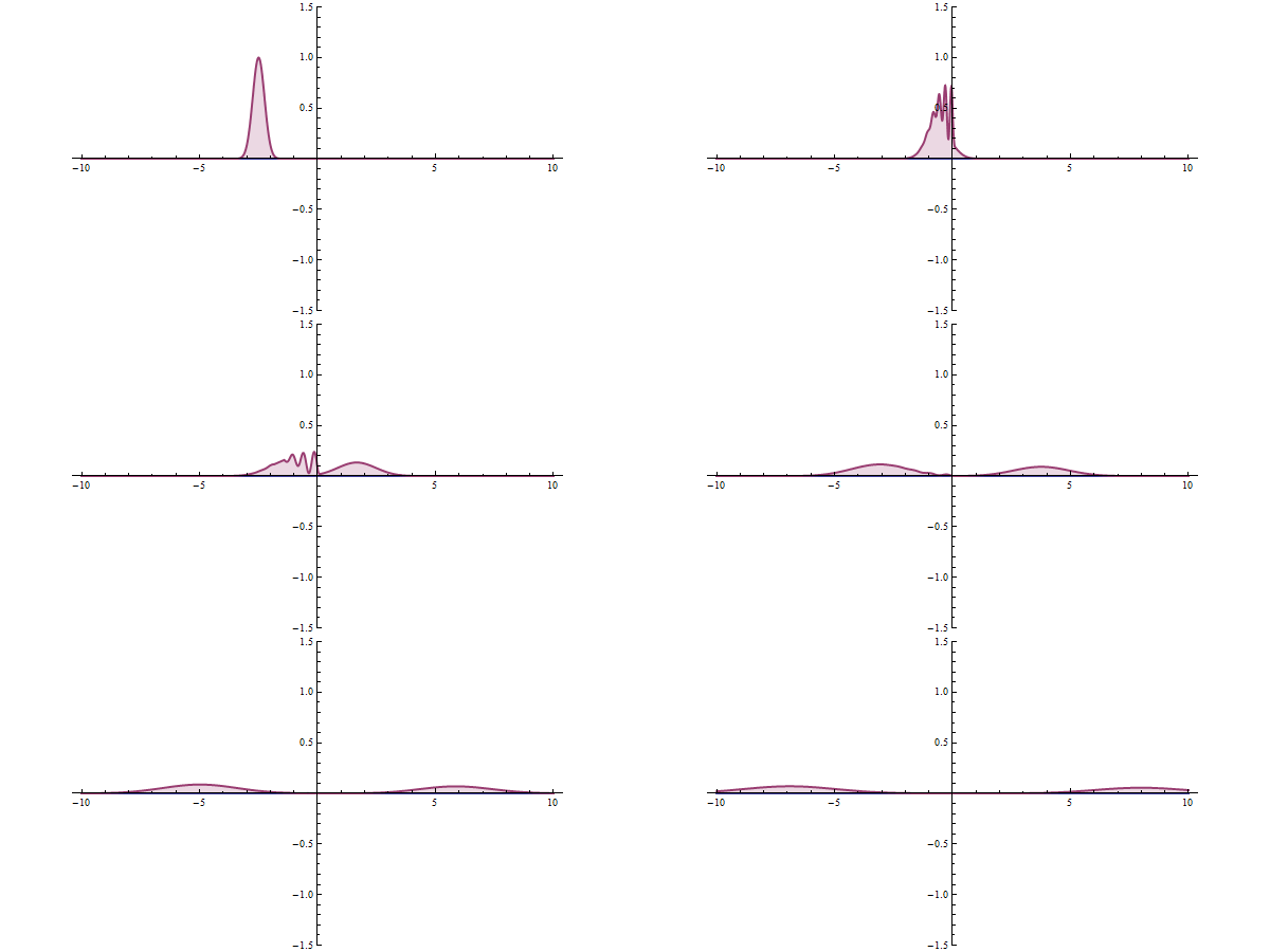
The derivation

Region 1 (x<0, V=0): incoming and reflected waves.

\psi_1 = Ae^{ikx}+Be^{-ikx}, \qquad k = \frac{\sqrt{2mE}}{\hbar}

Region 2 (0<x<a, V=V_0): the equation becomes

\frac{d^2\psi}{dx^2} = \frac{2m(V_0-E)}{\hbar^2}\psi = \kappa^2\psi, \qquad \kappa = \frac{\sqrt{2m(V_0-E)}}{\hbar}

Note the sign. With V_0 > E the right side is positive, so the solutions are real exponentials, not oscillations:

\psi_2 = Ce^{-\kappa x}+De^{\kappa x}

This is the whole of tunnelling in one line. The wavefunction does not stop at the barrier; it decays exponentially inside it. If the barrier is thin enough, the wavefunction has not decayed to nothing by the time it reaches the far side, and there it starts oscillating again.

Region 3 (x>a): transmitted wave only.

\psi_3 = Fe^{ikx}

Matching \psi and d\psi/dx at both boundaries gives four equations, and solving for |F/A|^2 gives the transmission probability. For a barrier that is not too thin (\kappa a \gg 1) it simplifies to:

\boxed{T \approx 16\frac{E}{V_0}\left(1-\frac{E}{V_0}\right)e^{-2\kappa a}}

The exponential is everything. The prefactor is of order 1; the physics is in:

T \sim e^{-2a\sqrt{2m(V_0-E)}/\hbar}

Three consequences follow directly:

• Exponentially sensitive to barrier width. Double the width and you square a small number.
• Exponentially sensitive to the mass. A proton is 1836 times heavier than an electron, so \sqrt{m} is 43 times larger and tunnelling is suppressed enormously. Electrons tunnel readily; nuclei rarely.
• Exponentially sensitive to barrier height.

Worked example: an electron through a nanometre

E = 1 eV, V_0 = 5 eV, a = 1 nm.

\kappa = \frac{\sqrt{2(9.109\times10^{-31})(4\times1.602\times10^{-19})}}{1.055\times10^{-34}} = \frac{\sqrt{5.836\times10^{-48}}}{1.055\times10^{-34}}

= \frac{2.416\times10^{-24}}{1.055\times10^{-34}} = 2.29\times10^{10}\ \text{m}^{-1}

2\kappa a = 2(2.29\times10^{10})(10^{-9}) = 45.8

T \approx 16(0.2)(0.8)e^{-45.8} = 2.56\times1.2\times10^{-20} = 3\times10^{-20}

Three in a hundred million million million. Now halve the barrier to 0.5 nm:

2\kappa a = 22.9, \qquad T \approx 2.56\,e^{-22.9} = 2.9\times10^{-10}

Ten orders of magnitude larger, from halving the width. That exponential sensitivity is what makes the scanning tunnelling microscope possible.

Where tunnelling runs the world

Alpha decay. An alpha particle inside a nucleus is trapped by the strong force but repelled by the Coulomb barrier outside. Classically it can never escape — its energy is a few MeV and the barrier is around 25 MeV. It tunnels.

George Gamow explained this in 1928, and it resolved a puzzle that had baffled physics for two decades: alpha decay half-lives span an enormous range, from 10^{-7} s for polonium-212 to 1.4\times10^{17} s for thorium-232 — a factor of 10^{24} — while the alpha energies vary by only a factor of two, from about 4 to 9 MeV.

The exponential explains it exactly. A small change in energy changes \kappa a little, and e^{-2\kappa a} changes enormously. The empirical relation, found by Geiger and Nuttall in 1911 with no explanation, is:

\log_{10}t_{1/2} = \frac{A}{\sqrt{E}}+B

and Gamow's tunnelling calculation produces exactly that form. This was the first application of quantum mechanics to the nucleus, and it was decisive.

Fusion in the Sun. Chapter 12.1 works this properly. The short version: the Sun's core is at 1.5\times10^{7} K, so the average proton has k_BT = 1.3 keV. To fuse, two protons must approach to about 1 fm, against a Coulomb barrier of:

V = \frac{ke^2}{r} = \frac{(8.988\times10^{9})(1.602\times10^{-19})^2}{10^{-15}} = 2.3\times10^{-13}\ \text{J} = 1.4\ \text{MeV}

The barrier is a thousand times the available thermal energy. Classically the Sun cannot shine at all. Even the far tail of the Maxwell–Boltzmann distribution (Chapter 3.2) does not close a factor of 1000.

Tunnelling closes it, at a rate so low that the Sun burns for ten billion years instead of exploding. The Sun's lifetime is set by how bad protons are at tunnelling.

Flash memory. A floating gate is surrounded by an insulator. Electrons are pushed onto it by tunnelling through the barrier when a high voltage is applied, and stay there because at normal voltages the tunnelling rate is negligible. Charge on the gate is a 1; no charge is a 0.

The exponential explains both the strength and the weakness. Data persists for years because the tunnelling rate at rest is astronomically small. And the memory wears out after 10^4 to 10^5 writes because each high-voltage pass damages the oxide, thinning it, and a thinner barrier leaks exponentially faster. Wear levelling in an SSD controller exists because of e^{-2\kappa a}.

Scanning tunnelling microscopy. Bring a sharp metal tip within a nanometre of a surface and apply a small voltage. Electrons tunnel across the gap, and the current depends exponentially on the distance — changing by about a factor of 10 for every 0.1 nm.

That sensitivity means essentially all the current flows through the single atom at the very end of the tip. Scan across the surface holding the current constant, and the tip's height traces the surface atom by atom. Binnig and Rohrer invented it in 1981 and had the Nobel Prize by 1986. In 1989 IBM used one to spell "IBM" in 35 xenon atoms.

Tunnel diodes and Josephson junctions are built directly on the effect, and the Josephson junction is the basis of the superconducting qubits used in most quantum computers.

And it limits chip manufacture. As transistor gate oxides thinned below about 2 nm, tunnelling leakage current became a serious fraction of a chip's power consumption. The industry's response was high-\kappa dielectrics — materials with a larger dielectric constant, so the same electrical effect is achieved with a physically thicker layer, which cuts the tunnelling exponentially. A 10^{-20} probability became a billion-dollar engineering problem.

The harmonic oscillator

Why this problem matters more than any other. Take any system sitting at a stable minimum of potential energy and expand around it (Chapter 2.1):

V(x) = V_0 + \frac{1}{2}V''(x_0)(x-x_0)^2 + \dots

The linear term vanishes at a minimum. So every stable system, to leading order, is a harmonic oscillator. Molecular bonds, crystal lattices, electromagnetic field modes, and the quantum fields of Chapter 7.10 all reduce to this.

The setup: V = \frac{1}{2}m\omega^2x^2.

-\frac{\hbar^2}{2m}\frac{d^2\psi}{dx^2}+\frac{1}{2}m\omega^2x^2\psi = E\psi

The result:

\boxed{E_n = \left(n+\tfrac{1}{2}\right)\hbar\omega, \qquad n = 0,1,2,\dots}

The quantum harmonic oscillator. The levels are evenly spaced, unlike the box's, and the lowest one sits half a step above the bottom of the well rather than at it. Image: Wikimedia Commons.

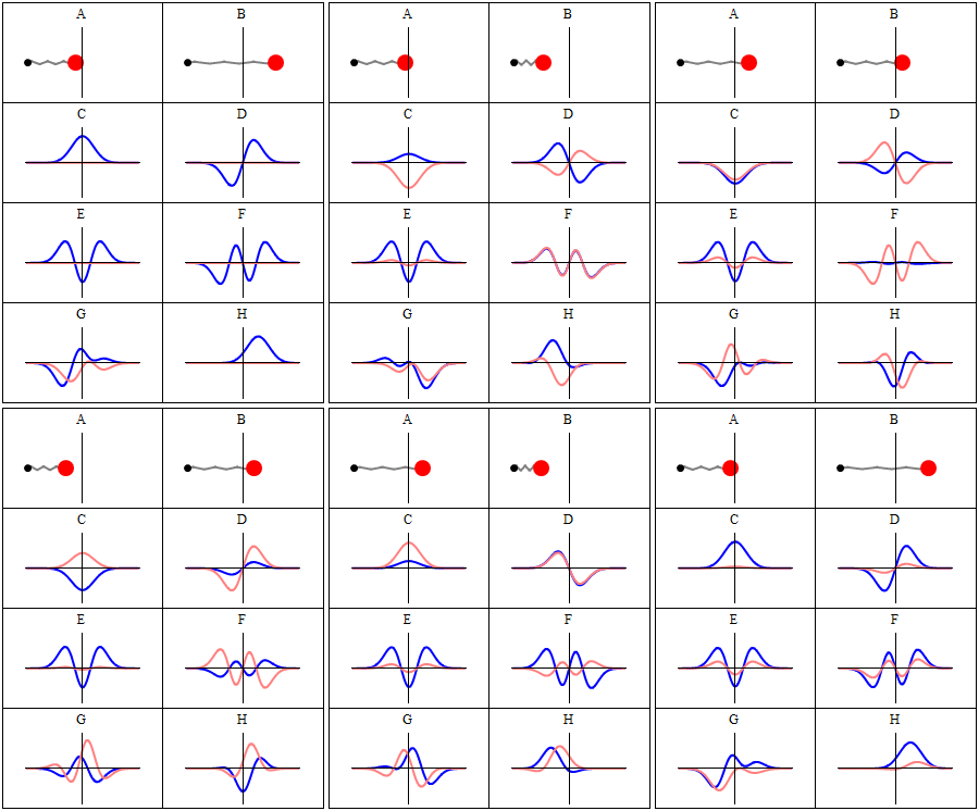
Three features, all consequential.

Evenly spaced levels. \Delta E = \hbar\omega between any adjacent pair. This is what Planck assumed in 1900 (Chapter 7.1) to fix the black-body catastrophe, and here it is derived rather than assumed. Planck's guess was exactly right about the spacing and wrong only in omitting the half.

Zero-point energy E_0 = \frac{1}{2}\hbar\omega. The lowest state is not at rest at the bottom of the well. Nothing is ever completely still, even at absolute zero. Chapter 7.9 pursues this.

The particle can be found where classical physics forbids it. In the ground state, about 16 % of the probability lies outside the classical turning points — the places where a classical oscillator of that energy would stop and turn back. It is the same exponential decay into a forbidden region as in tunnelling.

Worked example: a molecular bond

The hydrogen chloride molecule has a bond that vibrates at 8.66\times10^{13} Hz.

\Delta E = hf = (6.626\times10^{-34})(8.66\times10^{13}) = 5.74\times10^{-20}\ \text{J} = 0.358\ \text{eV}

The corresponding photon wavelength:

\lambda = \frac{hc}{E} = \frac{(6.626\times10^{-34})(3\times10^{8})}{5.74\times10^{-20}} = 3.46\times10^{-6}\ \text{m} = 3.46\ \mu\text{m}

Infrared — which is why infrared spectroscopy identifies molecules. Each bond type has its own vibrational frequency, so an infrared absorption spectrum is a list of which bonds are present. This is the standard identification method in every chemistry laboratory in the world.

And the zero-point energy:

E_0 = \frac{1}{2}(5.74\times10^{-20}) = 2.87\times10^{-20}\ \text{J} = 0.179\ \text{eV}

Compare with k_BT at room temperature, 0.026 eV. The zero-point energy is seven times the thermal energy, so this bond is in its vibrational ground state at room temperature and the vibration is frozen out — which is precisely the explanation Chapter 3.2 needed for the missing heat capacity.

Isotope effects come from this. Replace hydrogen with deuterium and the reduced mass roughly doubles, so \omega = \sqrt{k/\mu} falls by \sqrt{2} and the zero-point energy falls with it. Since the bond is deeper by that amount, deuterium bonds are harder to break, and reactions involving breaking a C–H bond can run several times slower with C–D. This kinetic isotope effect is a standard tool for working out reaction mechanisms, and it is entirely a zero-point-energy phenomenon.

The finite well and the periodic lattice

Two extensions worth naming.

A finite well — walls of finite height — has only a limited number of bound states, and the wavefunctions leak into the walls exponentially. A shallow enough well in three dimensions may have no bound state at all. This is why the deuteron is barely bound and the diproton does not exist, which turns out to control the rate of the first step of solar fusion (Chapter 12.1).

A periodic array of wells is a crystal. The allowed energies form continuous bands separated by gaps, and whether a material conducts depends entirely on whether the highest occupied band is full. Full band with a large gap: insulator. Partly full: metal. Full band with a small gap: semiconductor. Volume III, Chapter 2 builds the whole of electronics on this, and it is the box problem with the boundary conditions changed.

Where this shows up in your life

Your SSD stores data by tunnelling and wears out for the same reason.

QLED and quantum-dot displays use E \propto 1/L^2.

Infrared spectroscopy identifies plastics for recycling, checks drug purity, and measures atmospheric CO₂.

Smoke detectors contain americium-241, which alpha-decays by tunnelling.

The Sun shines because protons tunnel, and it shines slowly enough for life to have evolved because they are bad at it.

And the STM image of individual atoms — the first direct picture of an atom ever made — is a map of e^{-2\kappa a}.

What the next chapter fixes

Three problems have been solved, and the method has been ad hoc: write down an equation, apply boundary conditions, extract energies. What is missing is the general structure — what an observable is in quantum mechanics, why measurements give definite values from indefinite states, what determines which quantities can be known simultaneously, and where the uncertainty principle comes from. Chapter 7.5 builds that framework, and derives the uncertainty principle rather than quoting it.